Gödel! #6 An Introduction to Gödel’s Theorems Chapter 3 Part 2

3.4 More Definitions

Some definitions we’ll be using:

i. Given a derivation of from the axioms of a theory in our particular logical apparatus, we say that is a theorem of . Symbolically, .

ii. A theory is sound iff all of its theorems are true (ie: iff ‘s interpretaion makes them true).

iii. A theory is decidable iff the property of being a theorem of is effectively decidable, ie: given a sentence there is a mechanical procedure for determining whether . This expands our notion of decidability from sentences/properties to theories.

iv. A theory  decides a sentence iff either or .

v. A theory is negation complete  iff decides every sentence in its language.

vi. is  inconsistent iff for some sentence we have both and .

The book draws attention to the idea that a theory can be decidable, without being negation complete (ie: able to decide any sentence). For example, a theory whose language contains three terms and the lone axiom . This language is decidable by using a truth table to see if a sentence is a theorem (ie: follows from the axioms) but, for example, the sentence cannot be decided by the theory.

3.5 The effective enumerability of theorems

A neat little theorem:

Theorem 3.1 If is an axiomatized formal theorey then (i) the set of wffs of , (i’) the set of sentences of , (ii) the set of proofs constructible in , and (iii) the set of theorems of can each be effectively enumerated.

Proof sketch of (i) and (i’): This one is pretty trivial, since is constructed from a finite alphabet (by our definition of axiomatized formal theory), its wffs and sentences can be enumerated by listing the length-1 strings in alphabetical order, followed by the length-2 strings and so on.

Proof sketch of (ii): Since a proof is just a linear sequence of sentences, we can take our enumeration of sentences from (i’) and enumerate them. This is a bit more complicated, since there we’re basically forming finite strings (our proofs) over an infinite, but countable alphabet (our sentences). One way of doing this will result in an enumeration where all the even numbered proofs (starting at 0) are length-1, then every other odd number will be length-2 sentence, then every other remaining number will be a length-3 sentence, and so on, and you eventually squeeze every sentence into your enumeration. The details of this are tricky, but its the same general idea as enumerating a set of programs in a given programming language, or the set of all tuples. As we go along, we must use the mechanical procedure for determining whether something counts as a valid proof (built into our definition of an axiomatized formal theory) to check whether our proof is valid. If it isn’t then we don’t count it.

Proof sketch of (iii): As with (ii), only this time we only record the conclusions from our valid proofs.

The text draws attention to the idea that just because we can enumerate all of the theorems of a theory, doesn’t make that theory decidable. The gist of this idea is that given a sentence that isn’t a theorem, we can’t simply compare it to our list of theorems to see if it isn’t on there, due to the fact that our list is infinite and we won’t know when to stop checking.

3.6 Negation-complete theories are decidable

Despite the above, there is an important special case: negation-complete theories.

Theorem 3.2 Any consistent, axiomatized, negation-complete formal theory is decidable.

Proof: Since either or for any given , we can simply enumerate all of ‘s theorems until or shows up. If we get then it is a theorem, and if we get then since is consistent, we know is not a theorem.

This concludes chapter 3. Coming up next is a little bit about the language of arithmetic and using it to express numerical properties and relations. After that, in chapters 5 and 6 we return to Gödel’s theorems and see two new ways of making the incompleteness theorems apparent. I’ll likely skip chapter 7 as it simply spells out what’s coming up in later chapters, and then in chapters 8 and 9 we’ll talk about two specific theories of arithmetic: Baby Arithmetic () and Robinson Arithmetic ()

Gödel! #5 An Introduction to Gödel’s Theorems Chapter 3 Part 1

3 Axiomatized formal theories

Alright, cards on the table: I found this chapter kind of boring until around the end, so I’m just going to try and skim through it to get to the interesting parts.

3.1 Formalization as an ideal

Gödel’s theorems are statements about formal languages. Why do we care about formal languages? It’s pretty straightforward: formal languages allow us to ensure correctness by following specific rules regarding structure and syntax. In a natural language, such as English, you can have sentences with ambiguous meanings. For example:

“John knows a woman with a cat named Amy.”

could have two possible meanings: either John knows a woman who has a cat whose name is Amy, or John knows a woman named Amy who has a cat. This won’t upset us too much in our day-to-day lives. Usually the intended meaning can be inferred from context. But when we’re trying to prove something logically, this requires precision. Thus, we can use a formal language (such as first-order logic or even any given programming language) to create an unambiguous parsing of our sentences.

Even in proofs, mathematics or computer science, however, we don’t always use such rigorous formalization, as such precision can be tedious. What’s important in these cases is more to do with conveying an understanding of a concept. But the underpinnings of the formal language exists, and if one desired should be able to be spelled out with perfect rigour.

3.2 Formalized languages

Normally we are interested in interpreted languages, ie: ones with not just a syntax for deriving valid structures, but one where those structures have actual meaning. I could symbolize one version of the John/Amy sentence from above with but that sentence is meaningless unless I also inform you that means “ knows “, means “ is a woman”, means “ has a cat”, and mean “John” and “Amy” respectively.

Thus, we will define a language as being a pair where is a syntactically defined system of expressions and is an intended interpretation of those expressions.

Starting with : it will be based on a finite alphabet of symbols (I’m pretty sure you can get away with relaxing the requirement to an effectively enumerable alphabet, but the book says finite so we’ll go with finite). Some of these symbols will make up ‘s logical vocabulary, for example: connectives, quantifiers, parentheses, identity… Other symbols will constitute ‘s non-logical vocabulary: predicates and relations, functions, constants, variables… We will also need a system of rules for determining which sequences of symbols are well-formed formulae of (referred to throughough the text as its wffs).

For example, in first-order logic, our logical vocabulary is . Our non-logical vocabulary is a bit more complicated in that it needs to potentially address infinitely many variables. There are two ways to do this. The way I like to think of it is having which gives you an infinite set containing all of your variables , all of your -place predicates and all of your -place functions . But, of course, this results in an infinite alphabet of symbols. The book chooses to accomplish this by having your variables be something like which operates on a finite alphabet ( and ). In either case, we will typically just denote variables as , predicates as , functions as and so on. As stated in the previous section, we don’t always need to use perfect rigour but it’s important to understand how it would be accomplished. The union of the logical and non-logical vocabularies form the language’s alphabet. To see how first-order logic determines its wffs, see wikipedia. It is important for our purposes that determining whether a sentence is a wff is effectively decidable.

We then use to set the interpretation of our language. It cant do this by manually setting the truth conditions for each wff (there are too many of them). What it does, rather, is to determine the domain of quantification, the which terms are applied to particular predicates, and the rules for determining the truth of a sentence. For example, might set the domain of quantification to the set of people, set the value constants to Socrates and Plato respectively, and the meaning of the predicate to mean “is wise”. Then continues by indicating which predicates are true of terms predicates, for example that is true of both and . Finally, sets up rules for determining whether wffs are true. For example a wff of the form is true iff is true and is true. This can be tedious but straightforward. Again, however, it is important that this process be an effectively decidable one.

3.3 Axiomatized formal theories

The following things are required to construct an axiomatized formal theory :

(a) First, some wffs of our ‘s language are selected as its axioms. There must be an effective decision procedure to determine whether a given wff is an axiom of . This doesn’t mean that must have a finite number of axioms: we can have an axiom schema which tells us that sentences of such-and-such a form are axioms. For example, in Zermelo-Fraenkel set theory any wff of the form (where can be substituted for (essentially) any property) is an axiom, giving the theory infinitely many axioms.

(b) We also need some form of deductive apparatus or proof system in order to prove things in . I’ve talked about proof systems before and demonstrated two: truth tables and Fitch-style calculus. The exact system used for is irrelevant so long as it is effectively decidable whether a derivation from premises to a conclusion is valid. Note that this is different from having an effective procedure to actually create this derivation. All is has to do is determine whether a given proof which has been provided is valid for teh system.

(c) Thus, given an axiomatized formal theory , since we can effectively decide which wffs are -axioms, and whether a derivation in ‘s proof system is valid, it follows that it is also decidable whether a given array of wffs forms a -proof (ie: which proofs are sound in ).

(d) For the remainder of this book, when we discuss theories, what we really mean is axiomatized formal theories. Many times in logic “theory” simply means any collection of sentences, thus we must be careful to make this distinction here.

Next time we’ll finish up chapter 3 where it actually gets interesting.

Gödel! #4 An Introduction to Gödel’s Theorems 2.2

2.4 Effective enumerability

Similar to effective computability and effective decidability, effective enumerability describes which sets can be enumerated using a strictly mechanical procedure (such as our Turing machines described in secion 2.2). Now it is easy to imagine a program that enumerates a finite set: it just spits out the elements of the set and then halts. Consider the program:

This program will enumerate the set . But what does it mean to effectively enumerate an infinite set? Consider the program:

We can get an intuitive sense that this program will enumerate the set of all natural numbers, , but can we formalize the notion of a non-terminating program being used to enumerate an infinite set? This isn’t discussed in the book, but I like to think of it as follows:

A program is said to list an element iff there, after some finite number of steps of execution prints out . If lists every element in a set then is said to enumerate . Thus, is effectively enumerable iff there exists a program which enumerates it.

So in our program above, we can now see formally that every element of will be listed after exactly steps (if we ignore steps involved in managing the loop logic.

An interesting fact is that every finite set is enumerable. To observe this, consider a finite set . This set is then enumerable by the program:

Thus, given any finite set, we can in essence simply store every element in the set into memory and spit them out on demand.

2.5 Effectively enumerating pairs of numbers

What follows is a useful theorem that we will use time and time again.

Theorem 2.2: The set of ordered pairs of numbers is effectively enumerable.

Proof: Consider a table of ordered pairs of numbers:

We can use a computer to zig-zag through this table (in the order indicated by the arrows) which will eventually arrive at every possible combination. Since the table will be stored somehow in memory, we must generate it on the fly since we can’t operate on an infinite table, but we can make the table of arbitrarily large size and increase it as needed due to the infinite memory capabilities of our idealized computer system. Thus, we have created a program which enumerates the set .

QED

The book mentions that you can explicitly create a computable function that will do this without the use of the table, however it doesn’t go into details and even if it did, this exercise can be quite messy. The way I actually know how to do it doesn’t involve the table at all and actually goes the other way, . It looks like:

You can also define inverse functions such that , but this is complex and involves -calculus which I’m not ready to get into yet.

That wraps up chapter 2. Next time: axiomatized formal theories and why we should care.

Gödel! #3 An Introduction to Gödel’s Theorems 2.1

2.3 Enumerable sets

Another useful notion we will be using time and again is that of effective enumerability. As with effective decidability and effective computability, we will first explain what it means to be enumerable in principle, before moving on to the effectively so. Straight from the book:

A set is enumerable if its members can – at least in principle – be listed off in some order (a zero-th, first, second) with every member appearing on the list; repetitions are allowed, and the list may be infinite.

What this means is that you can give a (possibly infinite) list that will contain every single member of and each member is guaranteed to appear a finite number of entries into this list. The finite case is fairly obvious if (where denotes the empty set containing no elements) then trivially all elements of will appear on any list (say, the empty list containing no entries). If is larger, but still finite, we can imagine just going through each of the elements and listing them one by one. For example, is an enumeration of the finite set . Similarly, also enumerates , although with redundancies and not in a natural order.

The tricky case is infinite lists. The condition you need to pay special attention to in this instance is that each element of must appear a finite number of entries into the list. So, for example, the following lists each enumerate (where denotes the infinite set containing all natural numbers):

1. 
2. 
3. 

Notice that in each case (assuming our patterns hold) we can determine exactly how many entries into the list a given number will appear. In 1. is in the position. In 2. appears entries down the list if is even, and entries down if is odd. In the third example appears entries into the list. Note that to make the math easier, we start our counting at zero: thus, the left-most element listed is the “zero-th”, the next is the first, the next is the second and so on. Now 2. and 3. are contrived examples but the point they make is that each appears a finite number of entries into the list, and we can tell exactly how far into the list it is. Contrast that with the following non-examples:

1. 
2. 
3. 

In 1., all the odd numbers seem to appear an infinite number of places into the list. This clearly violates precisely what we’re looking at. In 2. there’s still an obvious pattern, but any number greater than 100 doesn’t seem to appear at all. Finally, in 3. there’s no clear pattern to how the numbers are being listed. It is entirely possible that this is the beginning of some valid enumeration, but without more information it’s impossible to tell. So despite the fact that is enumerable, none of these three lists are valid ways to do so.

So hopefully that gives you a bit of an intuitive notion of the idea of enumerability. For the more formally-inclined, here is how this is defined mathematically:

The set is enumerable iff either is empty or else there is a surjective (onto) function (so that is the range of ). We say that such a function enumerates .

The text proves that these two definitions are equivalent, but it’s fairly straightforward, so if you’re having trouble seeing it, I suggest sitting down and working out why these two versions of enumerability come out to the same thing. It should be similarly obvious that any subset of (finite or infinite) is also enumerable. However:

Theorem 2.1 There are infinite sets that are not enumerable.

Proof: Consider the set of infinite binary strings (ie: the set containing strings like ). Obviously is infinite. Suppose, for the purposes of contradiction (also known as reductio) that some enumerating function does exist. Then, for example, will look something like:

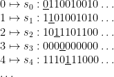
The exact values of aren’t important (as we will see) so this example will abstract to the general case. What we are going to do now is construct a new string, , such that does not appear in the enumeration generated by . We will do this by generating character-by-character. To determine the character in simple look at the character of and swap it. Thus, given our example enumeration above, the first 5 characters of would be which we get by just this method (for convenience, the character of each has been underlined). Now all we have to do is notice that will differ from each of the ‘s at precisely the position. As such, does not appear in the enumeration generated by . Thus, is not an enumeration of which contradicts our hypothesis that is enumerable.

QED

This gives us some interesting corollaries depending on how you want to interpret the set :

For example, a binary string can be thought of as representing a real binary decimal number (ie: would represent and would represent . Thus we know that the real numbers in the interval are not enumerable  (and so neither is the set of all real numbers ).

Another way to think of is that it is the set of sets of natural numbers. To see this, interpret a given string to be the set , where a number iff and iff . So for example, if then . Thus, the set of sets of natural numbers (denoted ) is also not enumerable.

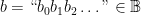
In later chapters we will learn the notion of a characteristic function which is a function which takes a numerical property and maps if holds and if holds. (This may seem backwards, since typically denotes and denotes , however we will see the reasons for this in due course.) If we consider an element to describe a characteristic function by , then we can observe that the set of all characteristic functions is similarly non-enumerable.

Next time we will finish up chapter 2 by discussing the limitations of what can be effectively enumerated by a computer program.

Gödel! #2 An Introduction to Gödel’s Theorems 2.0

2 Decidability and enumerability

Here we go over some basic notions that will be crucial later.

2.1 Functions

As I imagine anyone reading this is aware (although it’s totally cool if you’re not… that’s why it’s called learning), a function is a rule that takes something from its domain and turns it into something from its co-domain . We will be dealing exclusively with total functions, which means that is defined for every element in . Or, more plainly, we can use anything in as an argument for and have it make sense. This is contrasted with the notion of partial functions, which can have elements of the domain that isn’t designed to handle. We will not be using partial functions at any point in this book (or so it promises).

So, given a function , some definitions:

The range of a function is the subset of the that can possibly get to from elements of , ie: . In other words, the range is the set of all possible outputs of .

is surjective iff for every there is some such that . Equivalently, is surjective iff every member of its co-domain is a possible output of iff its co-domain and its range are identical. This property is also called onto.

is injective iff for it maps every different element of to a different element of . Equivalently, is injective iff implies that . This property is also called one-to-one because it matches everything with exactly one corresponding value.

is bijective iff it is both surjective and injective. Because is defined for every element of (total), can reach every member of (surjective) and matches each thing to exactly one other thing (injective), an immediate corollary of this is that and have the same number of elements. This is an important result that we will use quite often when discussing enumerability.

2.2 Effective decidability, effective computability

Deciding is the idea of determining whether a property or a relation applies in a particular case. For example, if I ask you to evaluate the predicate “is red” against the term “Mars”, you would say yes. If I gave you the predicate “halts in a finite number of steps” to the computer program you would probably say no. In either case you have just decided that predicate.

Computing is the idea of applying a function to an argument and figuring out the result is. If I give you the function and the argument you would compute the value . If I give you the function to the argument of the same computer program as above, you would conclude that the result is infinite. In both cases you have just computed that function.

What effectiveness comes down to is the notion of whether something can be done by a computer. Effective decidability is the condition that a property or relation can be decided by a computer in a finite number of operations. Effective computability is the condition that the result of a function applied to an argument can be calculated by a computer in a finite number of operations. For each notion, consider the two sets of two examples above. In each, the first is effectively decidable/computable and the second is not, for reasons I hope will eventually be clear.

This raises an obvious questions: what is a computer? Or, more to the point, what can computers do exactly? For our purposes we will be using a generalized notion of computation called a Turing machine (named for their inventor, Alan Turing). Despite its name, a Turing machine is not actually a mechanical device, but rather a hypothetical one. Imagine you have an infinite strip of tape, extending forever in both directions. This tape is divided up into squares, each square containing either a zero or a one. Imagine also that you can walk up and down and look at the square you’re standing next to. You have four options at this point (and can decide which to do take based on whether you’re looking at a zero or a one, as well as a condition called the “state” of the machine): you can either move to the square to your left, move to the square on your right, change the square you’re looking at to a zero, or change it to a one. It may surprise you, but the Turing machine I have just described is basically a computer, and can execute any algorithm that can be run on today’s state-of-the-art machines.

In fact, throughout the history of computability theory, whenever a new model has been developed of what could be done algorithmically by a computer (such as -calculus, -calculus, and even modern programming languages) it has turned out that each of these notions were equivalent to a Turing machine, as well as each other. Thus, Alan Turing and Alonzo Church separately came up with what is now called the Church-Turing thesis (although the book only deals with Turing, hence “Turing’s thesis”):

Turing thesis: the numerical functions that are effectively computable in an informal sense (ie: where the answer can be arrived at by a step-by-step application of discrete, specific numerical operations, or “algorithmically”)  are just those functions which are computable by a properly programmed Turing machine. Similarly, the effectively decidable properties and relations are just the numerical properties and relations which are decidable by a suitable Turing machine.

Of course we are unable to rigorously define an “intuitive” or “informal” notion of what could be computed, so Turing’s thesis could never be formally proven, however all attempts to disprove it have been thoroughly rebuked.

You might wonder, however, about just how long it might take such a simple machine to be able to solve complex problems. And you would be right to do so: Turing machines are notoriously hard to program, and take an enormous number of steps in order to solve most interesting problems. If we were to actually use such a Turing machine to try and get a useful answer to a question (as opposed to, say, writing a C++ program) it could very realistically take lifetimes to calculate. By what right, then, do we call this “effective”? Another objection to be raised might have to do with the idea of an infinite storage medium, which violates basic engineering principles of modern computer architectures.

Both of these objections can be answered at once: when we discuss computability, we are not so much interested in how practical it is to run a particular program. What interests us is to know what is computable in principle, rather than in practice. The reason for this is simple: when we discover a particular problem that cannot be solved by a Turing machine in a finite number of steps, this result is all the more surprising for the liberal attitude we’ve taken towards just how long we will let our programs run, or how much space we will allow them to take up.

One final note in this section. The way we’ve defined Turing machines, they operate on zeroes and ones. This of course reflects how our modern computers represent numbers (and hence why the Turing thesis refers to “numerical” functions, properties and relations). So how then can we effectively compute functions or decide properties of other things, such as truth values or sentences? This is simple. We basically encode such things into numbers and then perform numerical operations upon them.

For example, most programming languages encode the values of and as and , respectively. We can do the same thing with strings. An immediate example is ASCII encoding of textual characters to numeric values which is standardized across virtually all computer architectures. Later in the book we will learn another, more mathematically rigorous way to do the same.

The rest of this chapter is about the enumerability and effective enumerability of sets, but I’m going to hold off on talking about those until next time.

Gödel! #1 An Introduction to Gödel’s Theorems 1.0

I am going to rip off something Zach Weiner has been doing on his blog where he’s blogging his way through a few different textbooks. This sounds like an awesome way to get a better understanding out of stuff, so I am going to completely steal the idea from him, including the way he formats his titles (while giving him full credit as my inspiration) and blog my way through some of the textbooks I bought in university but never really actually bothered to crack open. Perhaps more fun for me than for you, but we’ll see how it goes.

The textbook I’m going to start off with is called An Introduction to Gödel’s Theorems written by Peter Smith. From the bits of it I’ve actually made use of, it’s a fairly detailed logic text while still being relatively accessible to anyone with a bit of background. Some of the concepts it seems to take for granted are elementary set theory, introductory logic, and basic computability theory. But most everything we’ll need seems to be covered in the text.

1 What Gödel’s Theorems say

1.1 Basic arithmetic

A lot of what is going to be covered in the text has to do with basic arithmetic, which is to say the natural numbers (0, 1, 2, etc…) and operations on them (addition, multiplication, etc…). Although this will all be flushed out formally in a few chapters, the natural numbers have a specific starting point, 0, each one has a unique successor, and every number falls into this sequence. But this will all be made formal in short order.

Our bigger concern is the notion of a formalized mathematics. In 1920 mathematician David Hilbert put forward a program to axiomatize all of mathematics into a set of finite, simple and non-controversial mathematical statements. The goal was to lift mathematics up by its bootstraps and prove the completeness and consistency of mathematics from these axioms in order to leave zero doubt as to their correctness.

The idea would be that mathematics could be axiomatized into a theory (a theory is simply a collection of axioms) that would be (negation) complete, which is to say that for any sentence , either or would be provable in .

Thus, in our case, we are considering how one could build a complete theory of basic arithmetic where we could prove (or disprove) conclusively the truth of any claim that could be expressed arithmetically. This is where Gödel’s Theorems come into play…

1.2 Incompleteness

… by basically shitting all over the idea. What mathematician Kurt Gödel was able to do in a 1931 paper was present a way to, given a theory which was sufficiently strong enough to express arithmetic, construct a sentence such that neither nor can be derived in , yet we can show that if is consistent then will be true.

Thus, basic arithmetic in its most striped-down form fails to be negation complete, which puts quite a dampener on Hilbert’s program.

The specifics of how is actually constructed is the subject of most of the text, but the gist of it is this: encodes the sentence “ is unprovable in “. Thus, is true iff can’t prove it. Suppose then that is sound (ie: cannot prove a false sentence). Then if it were to prove it would prove a falsehood, which violates soundness. Thus does not prove and so is true. Thus, is false, which means that can’t prove it either. Again, how is constructed is what we’ll be getting to, but this is the gist of Gödel’s First Theorem.

It should also be noted that there isn’t only one such sentence that renders incomplete. Suppose we decide to augment by adding to it, to create a new theory . We will then be able to construct a new Gödel sentence, which will be true but unprovable in . Since encompasses , will also be unprovable in and we get a construction of an infinite number of unprovable-in- sentences.

Thus, arithmetic is not only incomplete, but indeed incompletable.

1.3 More incompleteness

This incompletability does not just affect arithmetic. In fact it will also affect any systems which could be used to represent arithmetic. For example, set theory can define the empty set . Then, form the set containing the empty set, followed by the set containing both these sets and so on. We get a sequence of the form:

where we can define 0 as , 1 as the set containing 0, 2 as the set containing 0 and 1, and so on. The successor of is unioned with itself (ie: ), addition is defined as iterated succession, multiplication as iterated addition and all of a sudden you have a theory of arithmetic encompassed in set theory. By Gödel’s First Theorem, then, set theory is also incomplete.

1.4 Some implications?

This section deals with some philosophical implications of the First Theorem, but doesn’t delve into enough detail to be worth talking about.

1.5 The unprovability of consistency

Any worthwhile arithmetical theory will be able to prove the proposition . Thus, any decent theory that proves will be inconsistent. Furthermore, an inconsistent theory can prove any proposition, including , thus a theory of arithmetic is inconsistent iff proves . Now, we’ve already established that we can encode facts about the provability of propositions in , thus we have a way to encode the idea that can’t prove , which is to say that can express its own consistency. We’ll call the sentence that expresses this

From above, we’ve already seen that a consistent theory can’t prove . Since is itself the sentence that expresses its own unprovability, we can then express (in ) that if is consistent then is unprovable by .

Make sense?

According to the text, it turns out (although we’ve yet to see how) that this sentence turns out to be provable within theories with conditions only slightly stronger than those required for the First Theorem. However must still be unprovable within such theories, and so must also be unprovable otherwise we would be able to get by simple modus ponens.

As such, we have Gödel’s Second Incompleteness Theorem: that nice theories that can express a sufficient amount of arithmetic can’t prove their own consistency.

1.6 More implications?

The key point that I took from this section is that since we’ve shown that a theory of arithmetic can’t prove its own completeness or consistency, then it certainly can’t prove the same for a richer theory . This rudely defeats what remains of Hilbert’s Programme, as arithmetic isn’t capable of validating itself, let alone the rest of mathematics.

1.7 What’s next?

Obviously this is all pretty roughshod. In chapter 2 we go over a few basic notions that we will need to prove things in more detail. Chapter 3 discusses what is meant by an “axiomatized theory”. Chapter 4 introduces concepts specific to axiomatized theories of arithmetic. Chapters 5 and 6 give us some more direction as we head off towards formally proving… pause for dramatic music… Gödel’s First Incompleteness Theorem!