Gödel! #6 An Introduction to Gödel’s Theorems Chapter 3 Part 2

3.4 More Definitions

Some definitions we’ll be using:

i. Given a derivation of from the axioms of a theory in our particular logical apparatus, we say that is a theorem of . Symbolically, .

ii. A theory is sound iff all of its theorems are true (ie: iff ‘s interpretaion makes them true).

iii. A theory is decidable iff the property of being a theorem of is effectively decidable, ie: given a sentence there is a mechanical procedure for determining whether . This expands our notion of decidability from sentences/properties to theories.

iv. A theory  decides a sentence iff either or .

v. A theory is negation complete  iff decides every sentence in its language.

vi. is  inconsistent iff for some sentence we have both and .

The book draws attention to the idea that a theory can be decidable, without being negation complete (ie: able to decide any sentence). For example, a theory whose language contains three terms and the lone axiom . This language is decidable by using a truth table to see if a sentence is a theorem (ie: follows from the axioms) but, for example, the sentence cannot be decided by the theory.

3.5 The effective enumerability of theorems

A neat little theorem:

Theorem 3.1 If is an axiomatized formal theorey then (i) the set of wffs of , (i’) the set of sentences of , (ii) the set of proofs constructible in , and (iii) the set of theorems of can each be effectively enumerated.

Proof sketch of (i) and (i’): This one is pretty trivial, since is constructed from a finite alphabet (by our definition of axiomatized formal theory), its wffs and sentences can be enumerated by listing the length-1 strings in alphabetical order, followed by the length-2 strings and so on.

Proof sketch of (ii): Since a proof is just a linear sequence of sentences, we can take our enumeration of sentences from (i’) and enumerate them. This is a bit more complicated, since there we’re basically forming finite strings (our proofs) over an infinite, but countable alphabet (our sentences). One way of doing this will result in an enumeration where all the even numbered proofs (starting at 0) are length-1, then every other odd number will be length-2 sentence, then every other remaining number will be a length-3 sentence, and so on, and you eventually squeeze every sentence into your enumeration. The details of this are tricky, but its the same general idea as enumerating a set of programs in a given programming language, or the set of all tuples. As we go along, we must use the mechanical procedure for determining whether something counts as a valid proof (built into our definition of an axiomatized formal theory) to check whether our proof is valid. If it isn’t then we don’t count it.

Proof sketch of (iii): As with (ii), only this time we only record the conclusions from our valid proofs.

The text draws attention to the idea that just because we can enumerate all of the theorems of a theory, doesn’t make that theory decidable. The gist of this idea is that given a sentence that isn’t a theorem, we can’t simply compare it to our list of theorems to see if it isn’t on there, due to the fact that our list is infinite and we won’t know when to stop checking.

3.6 Negation-complete theories are decidable

Despite the above, there is an important special case: negation-complete theories.

Theorem 3.2 Any consistent, axiomatized, negation-complete formal theory is decidable.

Proof: Since either or for any given , we can simply enumerate all of ‘s theorems until or shows up. If we get then it is a theorem, and if we get then since is consistent, we know is not a theorem.

This concludes chapter 3. Coming up next is a little bit about the language of arithmetic and using it to express numerical properties and relations. After that, in chapters 5 and 6 we return to Gödel’s theorems and see two new ways of making the incompleteness theorems apparent. I’ll likely skip chapter 7 as it simply spells out what’s coming up in later chapters, and then in chapters 8 and 9 we’ll talk about two specific theories of arithmetic: Baby Arithmetic () and Robinson Arithmetic ()

Gödel! #5 An Introduction to Gödel’s Theorems Chapter 3 Part 1

3 Axiomatized formal theories

Alright, cards on the table: I found this chapter kind of boring until around the end, so I’m just going to try and skim through it to get to the interesting parts.

3.1 Formalization as an ideal

Gödel’s theorems are statements about formal languages. Why do we care about formal languages? It’s pretty straightforward: formal languages allow us to ensure correctness by following specific rules regarding structure and syntax. In a natural language, such as English, you can have sentences with ambiguous meanings. For example:

“John knows a woman with a cat named Amy.”

could have two possible meanings: either John knows a woman who has a cat whose name is Amy, or John knows a woman named Amy who has a cat. This won’t upset us too much in our day-to-day lives. Usually the intended meaning can be inferred from context. But when we’re trying to prove something logically, this requires precision. Thus, we can use a formal language (such as first-order logic or even any given programming language) to create an unambiguous parsing of our sentences.

Even in proofs, mathematics or computer science, however, we don’t always use such rigorous formalization, as such precision can be tedious. What’s important in these cases is more to do with conveying an understanding of a concept. But the underpinnings of the formal language exists, and if one desired should be able to be spelled out with perfect rigour.

3.2 Formalized languages

Normally we are interested in interpreted languages, ie: ones with not just a syntax for deriving valid structures, but one where those structures have actual meaning. I could symbolize one version of the John/Amy sentence from above with but that sentence is meaningless unless I also inform you that means “ knows “, means “ is a woman”, means “ has a cat”, and mean “John” and “Amy” respectively.

Thus, we will define a language as being a pair where is a syntactically defined system of expressions and is an intended interpretation of those expressions.

Starting with : it will be based on a finite alphabet of symbols (I’m pretty sure you can get away with relaxing the requirement to an effectively enumerable alphabet, but the book says finite so we’ll go with finite). Some of these symbols will make up ‘s logical vocabulary, for example: connectives, quantifiers, parentheses, identity… Other symbols will constitute ‘s non-logical vocabulary: predicates and relations, functions, constants, variables… We will also need a system of rules for determining which sequences of symbols are well-formed formulae of (referred to throughough the text as its wffs).

For example, in first-order logic, our logical vocabulary is . Our non-logical vocabulary is a bit more complicated in that it needs to potentially address infinitely many variables. There are two ways to do this. The way I like to think of it is having which gives you an infinite set containing all of your variables , all of your -place predicates and all of your -place functions . But, of course, this results in an infinite alphabet of symbols. The book chooses to accomplish this by having your variables be something like which operates on a finite alphabet ( and ). In either case, we will typically just denote variables as , predicates as , functions as and so on. As stated in the previous section, we don’t always need to use perfect rigour but it’s important to understand how it would be accomplished. The union of the logical and non-logical vocabularies form the language’s alphabet. To see how first-order logic determines its wffs, see wikipedia. It is important for our purposes that determining whether a sentence is a wff is effectively decidable.

We then use to set the interpretation of our language. It cant do this by manually setting the truth conditions for each wff (there are too many of them). What it does, rather, is to determine the domain of quantification, the which terms are applied to particular predicates, and the rules for determining the truth of a sentence. For example, might set the domain of quantification to the set of people, set the value constants to Socrates and Plato respectively, and the meaning of the predicate to mean “is wise”. Then continues by indicating which predicates are true of terms predicates, for example that is true of both and . Finally, sets up rules for determining whether wffs are true. For example a wff of the form is true iff is true and is true. This can be tedious but straightforward. Again, however, it is important that this process be an effectively decidable one.

3.3 Axiomatized formal theories

The following things are required to construct an axiomatized formal theory :

(a) First, some wffs of our ‘s language are selected as its axioms. There must be an effective decision procedure to determine whether a given wff is an axiom of . This doesn’t mean that must have a finite number of axioms: we can have an axiom schema which tells us that sentences of such-and-such a form are axioms. For example, in Zermelo-Fraenkel set theory any wff of the form (where can be substituted for (essentially) any property) is an axiom, giving the theory infinitely many axioms.

(b) We also need some form of deductive apparatus or proof system in order to prove things in . I’ve talked about proof systems before and demonstrated two: truth tables and Fitch-style calculus. The exact system used for is irrelevant so long as it is effectively decidable whether a derivation from premises to a conclusion is valid. Note that this is different from having an effective procedure to actually create this derivation. All is has to do is determine whether a given proof which has been provided is valid for teh system.

(c) Thus, given an axiomatized formal theory , since we can effectively decide which wffs are -axioms, and whether a derivation in ‘s proof system is valid, it follows that it is also decidable whether a given array of wffs forms a -proof (ie: which proofs are sound in ).

(d) For the remainder of this book, when we discuss theories, what we really mean is axiomatized formal theories. Many times in logic “theory” simply means any collection of sentences, thus we must be careful to make this distinction here.

Next time we’ll finish up chapter 3 where it actually gets interesting.

Gödel! #3 An Introduction to Gödel’s Theorems 2.1

2.3 Enumerable sets

Another useful notion we will be using time and again is that of effective enumerability. As with effective decidability and effective computability, we will first explain what it means to be enumerable in principle, before moving on to the effectively so. Straight from the book:

A set is enumerable if its members can – at least in principle – be listed off in some order (a zero-th, first, second) with every member appearing on the list; repetitions are allowed, and the list may be infinite.

What this means is that you can give a (possibly infinite) list that will contain every single member of and each member is guaranteed to appear a finite number of entries into this list. The finite case is fairly obvious if (where denotes the empty set containing no elements) then trivially all elements of will appear on any list (say, the empty list containing no entries). If is larger, but still finite, we can imagine just going through each of the elements and listing them one by one. For example, is an enumeration of the finite set . Similarly, also enumerates , although with redundancies and not in a natural order.

The tricky case is infinite lists. The condition you need to pay special attention to in this instance is that each element of must appear a finite number of entries into the list. So, for example, the following lists each enumerate (where denotes the infinite set containing all natural numbers):

1. 
2. 
3. 

Notice that in each case (assuming our patterns hold) we can determine exactly how many entries into the list a given number will appear. In 1. is in the position. In 2. appears entries down the list if is even, and entries down if is odd. In the third example appears entries into the list. Note that to make the math easier, we start our counting at zero: thus, the left-most element listed is the “zero-th”, the next is the first, the next is the second and so on. Now 2. and 3. are contrived examples but the point they make is that each appears a finite number of entries into the list, and we can tell exactly how far into the list it is. Contrast that with the following non-examples:

1. 
2. 
3. 

In 1., all the odd numbers seem to appear an infinite number of places into the list. This clearly violates precisely what we’re looking at. In 2. there’s still an obvious pattern, but any number greater than 100 doesn’t seem to appear at all. Finally, in 3. there’s no clear pattern to how the numbers are being listed. It is entirely possible that this is the beginning of some valid enumeration, but without more information it’s impossible to tell. So despite the fact that is enumerable, none of these three lists are valid ways to do so.

So hopefully that gives you a bit of an intuitive notion of the idea of enumerability. For the more formally-inclined, here is how this is defined mathematically:

The set is enumerable iff either is empty or else there is a surjective (onto) function (so that is the range of ). We say that such a function enumerates .

The text proves that these two definitions are equivalent, but it’s fairly straightforward, so if you’re having trouble seeing it, I suggest sitting down and working out why these two versions of enumerability come out to the same thing. It should be similarly obvious that any subset of (finite or infinite) is also enumerable. However:

Theorem 2.1 There are infinite sets that are not enumerable.

Proof: Consider the set of infinite binary strings (ie: the set containing strings like ). Obviously is infinite. Suppose, for the purposes of contradiction (also known as reductio) that some enumerating function does exist. Then, for example, will look something like:

The exact values of aren’t important (as we will see) so this example will abstract to the general case. What we are going to do now is construct a new string, , such that does not appear in the enumeration generated by . We will do this by generating character-by-character. To determine the character in simple look at the character of and swap it. Thus, given our example enumeration above, the first 5 characters of would be which we get by just this method (for convenience, the character of each has been underlined). Now all we have to do is notice that will differ from each of the ‘s at precisely the position. As such, does not appear in the enumeration generated by . Thus, is not an enumeration of which contradicts our hypothesis that is enumerable.

QED

This gives us some interesting corollaries depending on how you want to interpret the set :

For example, a binary string can be thought of as representing a real binary decimal number (ie: would represent and would represent . Thus we know that the real numbers in the interval are not enumerable  (and so neither is the set of all real numbers ).

Another way to think of is that it is the set of sets of natural numbers. To see this, interpret a given string to be the set , where a number iff and iff . So for example, if then . Thus, the set of sets of natural numbers (denoted ) is also not enumerable.

In later chapters we will learn the notion of a characteristic function which is a function which takes a numerical property and maps if holds and if holds. (This may seem backwards, since typically denotes and denotes , however we will see the reasons for this in due course.) If we consider an element to describe a characteristic function by , then we can observe that the set of all characteristic functions is similarly non-enumerable.

Next time we will finish up chapter 2 by discussing the limitations of what can be effectively enumerated by a computer program.

Gödel! #2 An Introduction to Gödel’s Theorems 2.0

2 Decidability and enumerability

Here we go over some basic notions that will be crucial later.

2.1 Functions

As I imagine anyone reading this is aware (although it’s totally cool if you’re not… that’s why it’s called learning), a function is a rule that takes something from its domain and turns it into something from its co-domain . We will be dealing exclusively with total functions, which means that is defined for every element in . Or, more plainly, we can use anything in as an argument for and have it make sense. This is contrasted with the notion of partial functions, which can have elements of the domain that isn’t designed to handle. We will not be using partial functions at any point in this book (or so it promises).

So, given a function , some definitions:

The range of a function is the subset of the that can possibly get to from elements of , ie: . In other words, the range is the set of all possible outputs of .

is surjective iff for every there is some such that . Equivalently, is surjective iff every member of its co-domain is a possible output of iff its co-domain and its range are identical. This property is also called onto.

is injective iff for it maps every different element of to a different element of . Equivalently, is injective iff implies that . This property is also called one-to-one because it matches everything with exactly one corresponding value.

is bijective iff it is both surjective and injective. Because is defined for every element of (total), can reach every member of (surjective) and matches each thing to exactly one other thing (injective), an immediate corollary of this is that and have the same number of elements. This is an important result that we will use quite often when discussing enumerability.

2.2 Effective decidability, effective computability

Deciding is the idea of determining whether a property or a relation applies in a particular case. For example, if I ask you to evaluate the predicate “is red” against the term “Mars”, you would say yes. If I gave you the predicate “halts in a finite number of steps” to the computer program you would probably say no. In either case you have just decided that predicate.

Computing is the idea of applying a function to an argument and figuring out the result is. If I give you the function and the argument you would compute the value . If I give you the function to the argument of the same computer program as above, you would conclude that the result is infinite. In both cases you have just computed that function.

What effectiveness comes down to is the notion of whether something can be done by a computer. Effective decidability is the condition that a property or relation can be decided by a computer in a finite number of operations. Effective computability is the condition that the result of a function applied to an argument can be calculated by a computer in a finite number of operations. For each notion, consider the two sets of two examples above. In each, the first is effectively decidable/computable and the second is not, for reasons I hope will eventually be clear.

This raises an obvious questions: what is a computer? Or, more to the point, what can computers do exactly? For our purposes we will be using a generalized notion of computation called a Turing machine (named for their inventor, Alan Turing). Despite its name, a Turing machine is not actually a mechanical device, but rather a hypothetical one. Imagine you have an infinite strip of tape, extending forever in both directions. This tape is divided up into squares, each square containing either a zero or a one. Imagine also that you can walk up and down and look at the square you’re standing next to. You have four options at this point (and can decide which to do take based on whether you’re looking at a zero or a one, as well as a condition called the “state” of the machine): you can either move to the square to your left, move to the square on your right, change the square you’re looking at to a zero, or change it to a one. It may surprise you, but the Turing machine I have just described is basically a computer, and can execute any algorithm that can be run on today’s state-of-the-art machines.

In fact, throughout the history of computability theory, whenever a new model has been developed of what could be done algorithmically by a computer (such as -calculus, -calculus, and even modern programming languages) it has turned out that each of these notions were equivalent to a Turing machine, as well as each other. Thus, Alan Turing and Alonzo Church separately came up with what is now called the Church-Turing thesis (although the book only deals with Turing, hence “Turing’s thesis”):

Turing thesis: the numerical functions that are effectively computable in an informal sense (ie: where the answer can be arrived at by a step-by-step application of discrete, specific numerical operations, or “algorithmically”)  are just those functions which are computable by a properly programmed Turing machine. Similarly, the effectively decidable properties and relations are just the numerical properties and relations which are decidable by a suitable Turing machine.

Of course we are unable to rigorously define an “intuitive” or “informal” notion of what could be computed, so Turing’s thesis could never be formally proven, however all attempts to disprove it have been thoroughly rebuked.

You might wonder, however, about just how long it might take such a simple machine to be able to solve complex problems. And you would be right to do so: Turing machines are notoriously hard to program, and take an enormous number of steps in order to solve most interesting problems. If we were to actually use such a Turing machine to try and get a useful answer to a question (as opposed to, say, writing a C++ program) it could very realistically take lifetimes to calculate. By what right, then, do we call this “effective”? Another objection to be raised might have to do with the idea of an infinite storage medium, which violates basic engineering principles of modern computer architectures.

Both of these objections can be answered at once: when we discuss computability, we are not so much interested in how practical it is to run a particular program. What interests us is to know what is computable in principle, rather than in practice. The reason for this is simple: when we discover a particular problem that cannot be solved by a Turing machine in a finite number of steps, this result is all the more surprising for the liberal attitude we’ve taken towards just how long we will let our programs run, or how much space we will allow them to take up.

One final note in this section. The way we’ve defined Turing machines, they operate on zeroes and ones. This of course reflects how our modern computers represent numbers (and hence why the Turing thesis refers to “numerical” functions, properties and relations). So how then can we effectively compute functions or decide properties of other things, such as truth values or sentences? This is simple. We basically encode such things into numbers and then perform numerical operations upon them.

For example, most programming languages encode the values of and as and , respectively. We can do the same thing with strings. An immediate example is ASCII encoding of textual characters to numeric values which is standardized across virtually all computer architectures. Later in the book we will learn another, more mathematically rigorous way to do the same.

The rest of this chapter is about the enumerability and effective enumerability of sets, but I’m going to hold off on talking about those until next time.

Gödel! #1 An Introduction to Gödel’s Theorems 1.0

I am going to rip off something Zach Weiner has been doing on his blog where he’s blogging his way through a few different textbooks. This sounds like an awesome way to get a better understanding out of stuff, so I am going to completely steal the idea from him, including the way he formats his titles (while giving him full credit as my inspiration) and blog my way through some of the textbooks I bought in university but never really actually bothered to crack open. Perhaps more fun for me than for you, but we’ll see how it goes.

The textbook I’m going to start off with is called An Introduction to Gödel’s Theorems written by Peter Smith. From the bits of it I’ve actually made use of, it’s a fairly detailed logic text while still being relatively accessible to anyone with a bit of background. Some of the concepts it seems to take for granted are elementary set theory, introductory logic, and basic computability theory. But most everything we’ll need seems to be covered in the text.

1 What Gödel’s Theorems say

1.1 Basic arithmetic

A lot of what is going to be covered in the text has to do with basic arithmetic, which is to say the natural numbers (0, 1, 2, etc…) and operations on them (addition, multiplication, etc…). Although this will all be flushed out formally in a few chapters, the natural numbers have a specific starting point, 0, each one has a unique successor, and every number falls into this sequence. But this will all be made formal in short order.

Our bigger concern is the notion of a formalized mathematics. In 1920 mathematician David Hilbert put forward a program to axiomatize all of mathematics into a set of finite, simple and non-controversial mathematical statements. The goal was to lift mathematics up by its bootstraps and prove the completeness and consistency of mathematics from these axioms in order to leave zero doubt as to their correctness.

The idea would be that mathematics could be axiomatized into a theory (a theory is simply a collection of axioms) that would be (negation) complete, which is to say that for any sentence , either or would be provable in .

Thus, in our case, we are considering how one could build a complete theory of basic arithmetic where we could prove (or disprove) conclusively the truth of any claim that could be expressed arithmetically. This is where Gödel’s Theorems come into play…

1.2 Incompleteness

… by basically shitting all over the idea. What mathematician Kurt Gödel was able to do in a 1931 paper was present a way to, given a theory which was sufficiently strong enough to express arithmetic, construct a sentence such that neither nor can be derived in , yet we can show that if is consistent then will be true.

Thus, basic arithmetic in its most striped-down form fails to be negation complete, which puts quite a dampener on Hilbert’s program.

The specifics of how is actually constructed is the subject of most of the text, but the gist of it is this: encodes the sentence “ is unprovable in “. Thus, is true iff can’t prove it. Suppose then that is sound (ie: cannot prove a false sentence). Then if it were to prove it would prove a falsehood, which violates soundness. Thus does not prove and so is true. Thus, is false, which means that can’t prove it either. Again, how is constructed is what we’ll be getting to, but this is the gist of Gödel’s First Theorem.

It should also be noted that there isn’t only one such sentence that renders incomplete. Suppose we decide to augment by adding to it, to create a new theory . We will then be able to construct a new Gödel sentence, which will be true but unprovable in . Since encompasses , will also be unprovable in and we get a construction of an infinite number of unprovable-in- sentences.

Thus, arithmetic is not only incomplete, but indeed incompletable.

1.3 More incompleteness

This incompletability does not just affect arithmetic. In fact it will also affect any systems which could be used to represent arithmetic. For example, set theory can define the empty set . Then, form the set containing the empty set, followed by the set containing both these sets and so on. We get a sequence of the form:

where we can define 0 as , 1 as the set containing 0, 2 as the set containing 0 and 1, and so on. The successor of is unioned with itself (ie: ), addition is defined as iterated succession, multiplication as iterated addition and all of a sudden you have a theory of arithmetic encompassed in set theory. By Gödel’s First Theorem, then, set theory is also incomplete.

1.4 Some implications?

This section deals with some philosophical implications of the First Theorem, but doesn’t delve into enough detail to be worth talking about.

1.5 The unprovability of consistency

Any worthwhile arithmetical theory will be able to prove the proposition . Thus, any decent theory that proves will be inconsistent. Furthermore, an inconsistent theory can prove any proposition, including , thus a theory of arithmetic is inconsistent iff proves . Now, we’ve already established that we can encode facts about the provability of propositions in , thus we have a way to encode the idea that can’t prove , which is to say that can express its own consistency. We’ll call the sentence that expresses this

From above, we’ve already seen that a consistent theory can’t prove . Since is itself the sentence that expresses its own unprovability, we can then express (in ) that if is consistent then is unprovable by .

Make sense?

According to the text, it turns out (although we’ve yet to see how) that this sentence turns out to be provable within theories with conditions only slightly stronger than those required for the First Theorem. However must still be unprovable within such theories, and so must also be unprovable otherwise we would be able to get by simple modus ponens.

As such, we have Gödel’s Second Incompleteness Theorem: that nice theories that can express a sufficient amount of arithmetic can’t prove their own consistency.

1.6 More implications?

The key point that I took from this section is that since we’ve shown that a theory of arithmetic can’t prove its own completeness or consistency, then it certainly can’t prove the same for a richer theory . This rudely defeats what remains of Hilbert’s Programme, as arithmetic isn’t capable of validating itself, let alone the rest of mathematics.

1.7 What’s next?

Obviously this is all pretty roughshod. In chapter 2 we go over a few basic notions that we will need to prove things in more detail. Chapter 3 discusses what is meant by an “axiomatized theory”. Chapter 4 introduces concepts specific to axiomatized theories of arithmetic. Chapters 5 and 6 give us some more direction as we head off towards formally proving… pause for dramatic music… Gödel’s First Incompleteness Theorem!

Classical Logic IV – First-Order Logic

(This is going to be a long one, but bear with me. Once we make it through this, I get to start talking about the cool stuff.)

4.1. Quantification

If you’ve been doing the questions for Parts II and III you may have run into some interesting quirks with symbolizing one of the arguments from Part I. Specifically:

• P1) All men are mortal.
• P2) Socrates is a man.
• C) Socrates is mortal.

Now, with a little bit of reflection, it’s clear that this argument ought to be valid. However, if we try to symbolize it using what you’ve already learned, we end up with something like:

• P1) R
• P2) S
• C) M

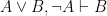
Which, it’s pretty clear, is not going to be a valid argument. The reason it doesn’t end up working out is because the basic logical language we’ve learned (known as Sentential or Propositional Logic) has no way of formalizing the concept of “all”.

That’s why there’s a second logical language that we’ll be talking about called First-Order Logic (or Predicate Logic). It is a strict extension of Propositional Logic, which is to say that everything you’ve already learned will still apply. (Well… you won’t be doing truth tables any more, but you won’t really miss them, I promise). In our extension we introduce two new concepts to our language: “some” and “all”. Because these describe quantities, they are called “quantifiers”.

4.1.1. Predicates

Before we learn about quantifiers, however, we need to discuss something called predicates. While they do have a fancy formal definition, I’d like to leave that for a future discussion and just cover them in an intuitive sense.

A predicate is like an adjective, in that it describes something about a subject. For example, in the sentence “a baseball is round”, the predicate “is round” describes a particular subject (in this case “a baseball”). Because we have separated the two things out, we can then go on to apply the predicate to other round things: “the Earth is round”, “circles are round” and “soccer balls are round” will, instead of each being their own sentence, be represented as a single predicate applied to three different round subjects.

Symbolically, we tend to denote predicates by uppercase letters, and subjects as lowercase letters. So in the examples above, we could let represent “is round” and then our four sentences become and (where represent “baseball”, “Earth”, “circles” and “soccer balls” respectively).

Typically however, we reserve letters from the beginning of the alphabet (,etc…) when we talk about particular subjects (called constants), and letters from the end of the alphabet (,etc…) when we talk about generic subjects (called variables).

4.1.2. Universal Quantification

So now that we have predicates, we can apply our first quantifier to it: the universal quantifier: . This symbol indicates that every subject has a particular property. In order to use it in a sentence, we must bind it to a variable such as . Once we’ve done this, we can create our sentence: or “everything is round”.

Now, this isn’t particularly helpful, since any useful predicate will be true of some things and not of others. That’s why we’re able to quantify over not just predicates, but other sentences. So, a more useful sentence might be which could be read as “anything which is a circle is also round”. In fact, we can even place a quantifier in front of a quantified sentence to end up with something like (which is a redundant sentence, but one that makes my point). Typically, we will abbreviate as .

In fact, this is the general form that most universal quantifications will take. For all if has some sort of property then has some other sort of property. To give another example, to say “all men are mortal” we would translate that as “all things that are men are mortal” or .

4.1.3. Existential Quantification

The other type of quantifier we can apply to a sentence is called an existential quantifier and is used to denote that some (or at least one) subject has a particular property. The symbol to denote this is and is used in a sentence exactly the same way as a universal quantifier: (read as “something is round”).

Again, this might not seem entirely useful, because it tells us nothing about what sorts of things the predicate applies to (in this case, what sorts of things are round?). But we can do another trick with them to narrow what we’re looking at by using conjunction. Take the predicate to mean “ is a plate$ then we have or “some plates are round”.

4.1.4. Relations

Relations are similar to predicates, except that they use more than one variable. For example, if you wish to say “James is the father of Harry”, we could take the predicate to describe a relationship between James () and Harry (). Symbolically we would write this as .

We aren’t just limited to two-place relations either. The predicate could represent the sentence “the priest married the husband and wife”. Examples with bigger and bigger relations do become more and more contrived, but technically speaking, there’s nothing to stop us.

We can also quantify over just part of a sentence. For example would say “someone is Harry’s father” and would say “James is the father of someone”.

Additionally, for two-place relations, they are sometimes represented with something called “infix notation”. Here, instead of saying we would write for whatever relation we’re dealing with. I prefer not to use this notation as it doesn’t work for relations with three or more subjects. With one notable exception:

4.1.4.1. Identity

We have the option of adding a special relation to our language, called identity (). It is a two-place relation written with infix notation that indicates that two things are the same. If we know that these two things are the same, then we can substitute one for the other in sentences. So the following sentence is valid (ie: always true) for any predicate :

Or, stated plainly, if two things are the same then any property that holds for one will also hold for the other.

I prefer to deal with first-order logic that makes use of identity, and so that is what I shall do. You may ask why we would choose not to do so, and the answer to that is basically just that it can make proving things about first-order logic a bit trickier. But that’s outside of the scope we’re dealing with here today.

Identity also has the following properties:

• Reflexivity:
• Symmetry:
• Transitivity:

Reflexivity tells us that everything is equal to itself. Symmetry tells us that it doesn’t matter which way we order our terms. Transitivity tells us that if one thing is equal to another, and the second thing is equal to some third, then the first and third things are also equal. These are the three properties that give us something called an equivalence relation, but we’ll get to what that is when we talk about set theory.

4.2. Socrates

With all of that under our belts, let’s look back at the original question. The argument:

• P1) All men are mortal.
• P2) Socrates is a man.
• C) Socrates is mortal.

Can now easily be symbolized as:

• P1)
• P2)
• C)

Easy enough, right? However this still doesn’t give us a way to tell whether the argument is valid. We can’t use a truth table, because there’s simply no way to express quantification in a truth table.  (Well technically we could, but only if we had a finite domain and even then it’s a pain in the ass…)

So we are still in need of a way to tell whether arguments in first-order logic are valid. Which brings us to…

4.2. Fitch-Style Calculus

There are a number of different ways to determine validity in first-order logic. I’m going to be talking about one called Fitch-Style Calculus, but there are many more including Natural Deduction (which I won’t be talking about) and Sequent Calculus and Semantic Tableaux (which I probably will).

I personally like Fitch because I find it very intuitive. A basic Fitch proof involves taking your premises and deriving a conclusion. We no longer deal with truth values, but instead we consider all of our assumptions to be true, but in a particular context. Just as an argument has two parts: premises and conclusions; so do Fitch proofs. These two parts are delimited by a giant version of the symbol. Premises (or assumptions) go on top of the symbol and conclusions go underneath. Additionally, each new line in your derivation must also be justified by a rule, which we’ll get to.

The most important concept in such derivations is that of the sub-proof. Basically a sub-proof is a brief argument-within-an-argument with its own assumptions which can be used within the sub-proof, but not in the outside proof as a whole. We will also make use of the term “scope” which basically refers to how many sub-proofs deep we are in a current argument. The rules (mentioned above) include ways to move sentences between different scopes.

I know this all sounds confusing, but we’re going to look at these rules and see whether they make sense. Before we do, I want to show you an example of a (admittedly complicated) proof, so that you can see what it looks like. You can check it out here. Take particular notice of the sub-proofs (and the sub-proofs within sub-proofs) to get an idea of how this sort of thing gets laid out. Also notice that each line is justified either as an assumption (appearing above the horizontal line of the symbol and abbreviated “Ass.” (try not to laugh)) or justified by a rule and the lines which the rule is making use of. Finally, notice that the last line is outside of any scope lines. We’ll see what this means later on.

But onto the rules! Once again, there are two different kinds: rules of inference and rewriting rules.

4.2.1. Fitch-Style Rules of Inference

Rules of inference are used to either introduce or eliminate a connective or quantifier from a sentence, or move sentences between scopes. They may require one or several lines earlier in the proof in order to make use of them. In the examples below, the line with the rule’s name next to it represents an application of that rule. Additionally, for these rules we will be using Greek letters to represent sentences which may not necessarily be atomic. This is because these rules are general forms which can be applied to very complex sentences. Thus, the symbol may stand for , , or even something as complicated as .

Each logical symbol in our language will have both an introduction rule (how to get that symbol to appear in a sentence) and an elimination rule (how to get it out). Thus, we have two rules each for plus one more, for a total of 19 rules.

4.2.1.1 Reiteration

The first rule of inference is kind of a silly one. Quite frankly, it almost always gets left out of written proofs (in fact, it’s been left out of my example proof above). Basically it states that any line of a proof can be repeated (reiterated) at any line within the same scope or deeper. In a proof, it looks something like:

Where basically you have some sentence and later on in the proof you repeat it. Notice that we are justifying the second appearance of it with the name of the rule: “Reit.” This is important to do in every line of your proof. Normally (as seen in my example proof) we also need to justify what lines the rule is being derived from. Because we have no line numbers here, they are omitted. There is a second (more useful, but still generally omitted) version of this rule which allows you to move a sentence into a sub-proof:

Notice however that although we can move sentences deeper into sub-proofs, we can’t take a sentence in a sub-proof and move it back outside of the sub-proof. In order to get things out of sub-proofs, we need different rules, which we’ll see shortly.

4.2.1.2. Conjunction Introduction and Elimination

These two rules are fairly straightforward. First, and-introduction:

This rule tells us that if we have two sentences, then we can simply “and” them together. Think of it this way: since we have and we have then we clearly have too.

And-elimination is simply the same thing, backwards:

If we have a conjunction, then we can derive either of the two terms. Put another way, if we have then we clearly must have and also .

4.2.1.3. Implication-Introduction and Elimination

Implication-introduction is the first time we will see the use of a sub-proof in one of our rules. It has the form:

This deserves a bit of explanation, but is pretty easy to understand once you see what’s going on. In our sub-proof, we are assuming . Now, it doesn’t actually matter whether is true or not, but for the sake of argument we are assuming that it is. Once we’ve done so, if we can somehow further derive then we are able to end the sub-proof (also called discharging our assumption) then we can conclude , which is just the formal way of saying “if then $psi$”, or “if we assume then we can conclude $\psi$”.

Implication elimination is identical to the Modus Ponens rule we learned in Part III. In fact, in many proofs (including my example proof above) we abbreviate the rule “MP” instead of “E”. To remind you, this rule has the following form:

As you can see, this is completely identical to what you learned about Modus Ponens earlier.

4.2.1.4. Disjunction Introduction and Elimination

Or-introduction is also fairly straightforward and takes the form:

Which is to say, if we have then we can loosen this to for any arbitrary sentence . Since disjunctions are also commutative (remember from Part III), we can also infer .

Or-elimination, on the other hand, is considerably more complex:

All this says, though is that if you have a disjunction and can derive the same sentence () from either disjunct, then regardless of whichever between or is true, must also hold. It is also important to notice that we are using two different sub-proofs. The sub-proof where we assume is completely separated from the one where we assume . So, for example, we couldn’t use the reiteration rule to bring into the second sub-proof because this would involve reiterating it to a less deep scope level. It can be a bit of a tricky one to wrap your head around, but once you’ve played around with it a bit, it begins to make sense.

4.2.1.5. Negation Introduction and Elimination

Negation introduction and elimination have exactly the same form. The only difference between the two is the location of the symbol:

In fact, we technically don’t even need both of these rules. Instead we could forgo the elimination rule and simply use the double negation rule (see below). We would do this by assuming , deriving , concluding using I and then rewriting it to using the double negation rule. If you understand what I just said, you’re doing great so far!

4.2.1.6. Biconditional Introduction and Elimination

These two rules basically just formalize the notion that a biconditional is literally a conditional that goes both ways. Its introduction rule has the form:

Where, if two sentences imply each other, then they mutually imply each other. The elimination rule has the form:

Where, if two things mutually imply each other, then they each imply the other on their own.

4.2.1.7. Bottom Introduction and Elimination

Recall that the symbol is a logical constant which represents a sentence which is always false. Basically, its only use is to enable the negation introduction and elimination rules. You might wonder how we could possibly derive a sentence which is always false when we’re assuming that our sentences are always true. Well that’s kind of the point. Observe:

The only way to actually derive is to derive a contradiction. This will usually only happen in the context of some sub-proof which allows us to use the negation introduction and elimination rules that say basically “if your assumption leads to a contradiction, then your assumption is incorrect”. This is also a form of argument which is known as “reductio ad absurdum” where you grant an opponent’s premise to show that it is logically inconsistent with some other point.

The bottom elimination rule does exist, but is seldom used. It has the form:

All this does is return us to the notion that anything is derivable from a contradiction. Regardless of what actually is, if we already have a contradiction, we can infer it. It’s not like we can make it more inconsistent!

4.2.1.8. Substitutions

Once we start involving quantifiers in our sentences, our rules start getting a bit muckier, because we have to deal not only with sentences containing predicates, but also terms. Because of this, we need to have something called a substitution, which I’ll explain briefly.

As the name suggests, a substitution takes one term out of a sentence and replaces it with a completely different term. This is written as where is some arbitrary sentence, is the term we are replacing, and is what we are replacing it with. Here are some examples:

• evaluates to
• evaluates to
• evaluates to
• evaluates to
• evaluates to

We may sometimes wish to talk about what terms appear in a sentence. I will use the notation to mean that the term appears in the sentence and the notation to mean that it does not. With that in mind, let’s move on.

4.2.1.9. Existential Introduction and Elimination

Existential introduction is a way to weaken a particular statement. It takes the form:

At any given time, we can take a concrete statement and make it abstract. To give a particular example, if we had the claim “the Earth is round” we could weaken it to say “something is round”. Which, while less helpful, is still true. We must, however, take care that the variable we are attaching to our quantifier does not already appear in our sentence. For example, if one had the sentence , we could derive but not , because already appears in our formula.

Existential elimination is a bit more straightforward, but also has a bit more bookkeeping involved with it:

If we know that there is some for which is true, then we can give it a concrete name. The only thing we have to be careful about is what name we give it. In general, we can’t give it a name that is already assigned to an item. So if we had and then we could derive . Once we’ve done so, however, we can no longer derive but we can derive (assuming has not already been used somewhere else within the same scope). A constant term that has not yet been used is called “fresh”.

4.2.1.10. Universal Introduction and Elimination

Universal introduction is weird, to the point where I don’t like to use it because it’s confusing. In the example proof I linked to above, I actually avoid using it and instead use a combination of negation elimination and a version of  DeMorgan’s laws (see below). But for the sake of completeness, here it is:

Once again, we have to make sure that the variable we are binding to our quantifier doesn’t appear in the rest of our sentence. But there’s another catch to this rule: in order to use it, you must be outside of any scope lines on your proof. In my example proof above, I could have used this rule to make another line at the end of the proof, but at no other point in my proof would this rule have been viable.

Universal elimination is much more straightforward:

We don’t have to worry about fresh variables or scope lines or anything else. Because is true for all we can just substitute whatever the hell we want in for . Easy.

4.2.1.11. Identity Introduction and Elimination

Our last (yay!) rule of inference involves the identity relation. Remember that this is a relation between two terms that indicates that they refer to the same entity. The introduction rule is as follows:

… wait, that’s it? Yep. Without having anything in advance, you can always deduce that any arbitrary term is identical to itself. No baggage required. The elimination rule is a bit more complicated, but really not by much:

If two things are identical, then they can be substituted for each other in any arbitrary sentence ().

4.2.2. Fitch-Rewriting Rules

The following rules allow you to rewrite sentences (or parts of sentences) in Fitch-style derivations. Actually, these rules will pretty much apply to any system of first-order logic. Once again, if you replace the with a biconditional then the resulting sentence is a tautology and will always be valid. Next time, I’ll even teach you how to prove this.

4.2.2.1. Commutativity

As we saw in Part III conjunction, disjunction and biconditionals are all commutative. Thus we have the following rewriting rules:

Additionally, the variables in a repeated existential or universal quantification are also commutative. This gives us:

It is important to note, however, that the following are not rewriting rules:

There’s an enormous difference between saying “everyone loves someone” and “someone loves everyone”, which is why the order of terms can only be arranged if they are under the same quantifier.

4.2.2.2. Associativity

Again, as we saw in Part III conjunction, disjunction and biconditionals are associative, meaning that it doesn’t matter what order you evaluate them in:

There’s no real difference here between propositional and predicate logics.

4.2.2.3. DeMorgan’s Laws

Also as seen in Part III, we have DeMorgan’s laws which identify the relationship between conjunction, disjunction and negation and allow us to define them in terms of each other.

However, we also have a variation DeMorgan’s Laws which operate on quantifiers:

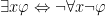
Seriously think about these until they make sense to you. It may help to think of an existential statement as a giant disjunction (ie: “something is round” means “either electrons are round or the Earth is round or squares are round or birds are round…”) and a universal statement as a giant conjunction (ie: “electrons have mass and the Earth has mass and squares have mass and birds have mass”).

4.2.2.4. Double Negation

Double negation is another one that’s straight out of last time:

If isn’t not true, then it must be true. Simple.

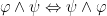
4.2.2.5. Definition of

Once again, can be defined in terms of and as follows:

Make sure you understand why this is true as well.

4.2.2.6. Symmetry and Transitivity of Identity

Finally, we have a couple of rules regarding identity. The first is easy enough:

You might ask yourself why this doesn’t fall under commutativity and the answer is a little bit confusing. Commutativity is a rule which applies between sentences. It says that you can swap the order of the sentences on either side of certain connectives. Symmetry is slightly different. It says that you can swap the order of the terms on either side of certain relations. It’s a bit of a technical distinction, but it’s one that’s important to maintain.

Transitivity of identity isn’t really a re-writing rule, but I like to put it here with symmetry because they go well together. Basically it states that if you know that and also that then you can also conclude that . It can be made into a rewriting rule by:

4.3. Future and Questions

It turns out that there’s actually a lot that needs to be said about first-order logic. As such, I’m going to split it into two (well, two-and-a-half) different entries. Next time I’ll talk about proving validity using Fitch-style systems as well as some strategies for proving things in first-order logic and translations of more complicated sentences. I also want to go over my example derivation and explain step-by-step what’s going on (in fact, I’ll probably do that part first).

In the meantime, here is a handy reference for all of the rules we went over today. See if you can answer the following questions:

1. Translate the following sentences into first-order logic:
• All circles are round.
• Some buildings are tall.
• Phil said hello to everyone at the market.
• Joe knows a guy who can get you cheap concert tickets.
• She is her mother’s daughter.
• She got married to someone who owned a farm.
• John is taller than Suzie, but shorter than Pete. Frank is taller than all of them.
• There is at least one apple in that basket.
• There are exactly two apples in that basket.
• There are no more than three apples in that basket.
2. Let be the sentence “ owns a tractor”. Translate the following sentences:
• 
• 
• 
• 
• 
• 
• 
• 
3. Determine whether the following relations are reflexive, symmetric and/or transitive:
• “is the father of”
• “is related to”
• “is an ancestor of”
• “is the brother of”
• “is the sibling of”
• “is descended from”
4. Without using any rewriting rules, use Fitch-style derivations to prove the tautological form of each of the rewriting rules (ie: replace “” with ““.
5. Use Fitch-style derivations to prove the following arguments:
• 
• 
• 
• 
• 
• 

Classical Logic III – Rules of Inference

3.1. Validity and Truth Tables

So it’s all well and good to be able to symbolize the sentences in an argument, but how does that help us when we’re trying to determine validity? Well let’s look at two related concepts that we’ve just learned and see if that can help us.

Remember the truth table for ? It’s okay if you don’t, I’ll give it to you here:

T	T	T
T	F	F
F	T	T
F	F	T

So basically, an implication is false only when the antecedent is true and the consequent is false.

Does this sound familiar? What was our definition of validity again? If it is impossible for the premises to be true, and the conclusion false, then the argument is valid. Can you see the connection? True implications have get true consequents from true antecedents and valid arguments get true conclusions from true premises. So how can we use truth tables to prove an argument is valid? Consider an example:

The argument:

• If it rains, then the grass will be wet.
• It is raining.
• Therefore, the grass is wet.

Can be symbolized as:

• P1) 
• P2) 
• C) 

But consider the sentence: where what we’ve done is taken the conjunction of the argument’s premises and then stated that they imply the argument’s conclusion. Let’s examine the truth table for this sentence:

T	T	T	T	T
T	F	F	F	T
F	T	T	F	T
F	F	T	F	T

Notice that, regardless of the truth values of and , our final sentence turns out to always be true. But consider what that sentence means: that the premises of our argument imply our conclusion. Since the sentence is always true, this means that the premises necessarily imply the conclusion. And this is simply a definition of validity.

So, in general, if we want to determine whether an argument is valid, we can use this method of creating a sentence by making a conjunction of our premises, and using that as the antecedent in an implication, with the conclusion as the consequent. Then simply make a truth table for that sentence, and if it holds in all possible truth assignments, we know we have a valid argument. Neat!

Let’s quickly look at an invalid argument, just so that you can see the difference. This sort of example is called a non-example and is often useful for visualizing what you’ve just learned. Consider the argument:

• P3) If it rains, the grass will be wet.
• P4) The grass is wet.
• C2) Therefore, it is raining.

As we discussed in Part I, this argument is invalid. So let’s symbolize the whole argument as and examine the resulting truth table.

T	T	T	T	T
T	F	F	F	T
F	T	T	T	F
F	F	T	F	T

Uh-oh… It looks like when is false and is true, the whole argument falls apart. Consider what this means: it is not raining, but the grass is still wet. This was exactly the reasoning we gave in Part I for why this was invalid. Neat how that works out. So given that, a valid argument must always have its resulting implication evaluate to true.

3.2. Rules of Inference

So we now know that some arguments are valid, some are invalid, and we can determine which are which by using truth tables. But the problem with deciding which arguments are valid that is you need to what their conclusions are ahead of time. This is not how critical thinking works. Usually we just want to start out with a few premises and see where these get us, while preserving the validity of what you come up with. This process is called inference or deduction, and can use a number of rules in order to pull it off. Let’s take a look at some of them:

3.2.1. Modus Ponens

Modus Ponens (or MP) is one of the most common tools in deduction, and says the following. If you have premises of the form $\latex A\rightarrow B$ and then you are able to conclude . Visually, we write this as:

Where the symbol is read as “entails” and means that if all the sentences on the left are true, then so is the sentence on the right. Or, put another way, if we know the sentences on the left, then we are able to deduce the sentence on the right.

This isn’t just some crazy thing I made up either: you can check whether it’s true or not… by using a truth table!

T	T	T	T	T
T	F	F	F	T
F	T	T	F	T
F	F	T	F	T

The right-hand column is always true, so MP must be a valid form of argument! In fact, if you look closely, this is the exact same table from our example of a valid argument above: you’ve already been using MP and you didn’t even know it!

It’s good practice to try making these tables, so I’m going to leave them out for the rest of this section. But don’t let that fool you: you should absolutely try to make them yourself. It’s important to be able to do this kind of stuff if you have any interest in logic.

3.2.2 Modus Tollens

Modus Tollens (MT) is kind of the reverse of MP in that it takes an implication and the truth value of the consequent in order to infer the truth value of the antecedent. Its logical form is:

Put another way, the only time that an implication can have a false consequent is when the antecedent is also false. Thus, we can infer that this is the case. Try doing the truth table for it. Seriously.

3.3.3. Disjunctive Syllogism

Disjunctive Syllogism (DS) says that, given a disjunction, if one of the disjuncts is false, then the other one must be true. This technically has two forms:

This one can be tricky to visualize, but if you do the truth table it becomes fairly obvious as to why this is valid. Doooo iiiitttt!

3.3.4. “And” Elimination

“And” Elimination (E) is a rule that states that if a conjunction is true, then so are its conjuncts. It also technically has two forms:

There’s not much to say about this one: if two things are true together, then obviously both of them are true on their own.

3.3.5. “And” Introduction

Similarly, if two things are true on their own, then both of them will be true together. This is what “And” Introduction (I) states.

3.3.6. “Or” Elimination

Okay, this one’s a bit weird. Bear with me. First I’m going to give you its logical form:

“Wait, where did this  business come from?” I hear you asking. Well if all we have to work from in an “Or” Elimination (E) is a single disjunction, then there’s not really any way of figuring out which of the two disjuncts are true. BUT! If we know that (whatever it happens to be) is implied by both and then regardless of which one is actually true, will hold either way.

It’s confusing, I know. That’s why you’re supposed to be doing the truth tables for these. Honestly, they make sense once you do.

3.3.7. “Or” Introduction

Not nearly as complicated is “Or” Introduction (I). It has the forms:

Again, springs out of nowhere, but it kind of makes sense this time. If we know that is true, then we can attach whatever we want to it without making a difference, so long as we’re saying that what we’re attaching is either true, or is (which it is).

3.3.8. “Iff” Elimination

If you’ll recall from Part II, “iff” is a short hand for “if and only if” and is used to describe the connective . Thus, “Iff” Elimination (E) is:

Which basically formalizes the idea that a biconditional indicates that both sides imply eachother.

3.3.9. “Iff” Introduction

“Iff” Introduction ($\leftrightarrow$I) is just the reverse of E and states:

Plainly, if two sentences imply each other, then they are equivalent.

3.3.10. Tautology

A tautology is a sentence which is always true. The canonical example is , since no matter what, exactly one of those will always be true (making the whole thing true). Other ones include or many more, which we’ll see below. But the neat thing about tautologies is that they can be inferred from nothing:

Remember that this means that if everything on the left is true (which it always will be, trivially) then the sentence on the right will be true (which it always will be, again)

This actually gives us a new notion of validity for sentences instead of arguments. A sentence is valid if and only if it is true under all truth value assignments. This also means that an argument can be said to be valid if and only if its logical form is valid.

3.3.11. Reductio ad Absurdum

Recall in Part I where we talked about how anything can be derived from a contradiction? Well we actually have a rule of inference for that. In fact, we have two, which can fall under the name Reductio ad Absurdum. The first one we will call I (or “Bottom Introduction”):

The symbol is called “bottom” and is a logical constant used to represent a contradiction. It is also used to represent a sentence which is always false, regardless of truth values (kind of like the opposite of a tautology), but these concepts are actually identical. You can even make a truth table to prove it.

The second rule is Bottom Elimination (E) and has the form:

Which is how we formalize our notion that anything can be derived from a contradiction.

This whole process is what’s referred to as Reductio ad Absurdum which is a form of argument where you assume something is true, in order to show that it leads to a contradiction, and thus can’t actually be true. But we’ll deal with this further in a more philosophically-minded post.

3.3.12. Summary

Because it’s handy to have that all in one place:

(MP)
(MT)
(DS)
(DS)
(E)
(E)
(I)
(E)
(I)
(I)
(E)
 (E)
 (I)
(Taut.)
(I)
(E)

3.4. Rewriting Rules

In addition to the rules of inference, there are many other rules which can be used to rewrite sentences (or even parts of sentences) in order to make derivations easier.

I like to call these rewriting rules. The interesting thing about them is that they can, themselves, all be rewritten take the form of a biconditional tautology. I’ll show you how at the end. For now, here are some useful rewriting rules:

3.4.1. Commutativity

Commutativity is a general math term used to indicate that it doesn’t matter what order your terms are in. For example, tells us that addition is commutative, since it doesn’t matter whether the or the comes first.

Similarly, classical logic has two main commutative operators: and . Our rewriting rules can be written as:

I am using the symbol to indicate that the left side can be rewritten as the right side, and vice versa, without affecting the truth of the sentence.

Now, this might seem obvious, but the reason it’s important to point out is that, while and are commutative, not everything else is. In particular is not. In order to see this, remember when we discussed the difference between “if” and “only if” in Part II.

3.4.2. Associativity

Associativity is another math term that indicates that it doesn’t matter what order you perform an operation in. Again, consider addition:

It doesn’t matter whether we add and first, or whether we add and . That’s why you would be more likely to see this kind of expression simply written as .

Similarly, and are both associative:

Which is why you will always see a string of ‘s and ‘s written without brackets as:

Again, for an example of an operator that is not associative try making truth tables for the sentences and .

3.4.3. DeMorgan’s Laws

DeMorgan’s Laws are probably the rewriting rules that you will use most often. They firmly establish the relationship between and . They are:

This can be easily remembered as “the negation of a conjunction is a disjunction of negations” and vice versa. But seeing why it’s this way is a lot harder. If you haven’t been doing the truth tables up until now, I very strongly encourage you to do this one, as this concept will come up time and time again, and not just in classical logic. It comes up in set theory, quantificational logic, modal logic: you name it! So do the truth tables now and get it out of the way. 🙂

3.4.4. Double Negation

Remember in Part I when I said that anything that isn’t true is false and anything that isn’t false is true? It may have seemed like a stupid thing to say at the time, but here’s why it’s important to point out: because it gives us this rule.

This should be clear enough: if a negation swaps the truth value of a sentence, then its negation should swap the truth value back to what it originally was. Easy, right? See, not all of these have to be painful.

3.4.5. Implicational Disjunction

I’ll level with you, I don’t actually know what this is called, and I couldn’t even find anything online naming it. But it’s important. Super important. This rule is:

In fact, this is so important that many logical systems don’t even bother defining implication, as you can get it simply with negation and disjunction. We’ll see why you might want to do this in the future, but for now just know that these two sentences are equivalent, and it can save you a lot of headaches. This is another one that I would strongly encourage you to do the truth table for.

3.4.6. Rewrites Are Tautologies

I mentioned above that rewriting rules can be rewritten as tautologies (sentences which are always true). Hopefully you’ve already figured this out, but in case you haven’t, in order to do this all you have to do is change into and BAM! You have a new sentence which will always be true.

No kidding, try it out!

3.4.7. Internal Rewrites

The biggest difference between rewriting rules and rules of inference is that rewriting rules can be used on the inside of sentences. For example:

Can be rewritten as:

Whereas, in order to apply a rule of inference, the entire sentence needs to have the relevant form.

3.4.8. Summary

And once again, because it’s handy to have them all in one place:

(Comm.)
 (Comm.)
 (Assoc.)
 (Assoc.)
 (DeM)
 (DeM)
(DN)
(def)

3.5. Questions

You should now be able to answer the following questions.

1. Use truth tables to show whether the arguments from Part I are valid in classical logic.
2. Create truth tables showing that all of the rules of inference from section 3.2. are valid.
3. Give three examples of tautologies.
4. Give three examples of contradictions.
5. Create truth tables showing that all of the rewriting rules from section 3.3. are valid.
6. Without creating a truth table, use DeMorgan’s Laws and Double Negation to show that:
• is equivalent to
• is equivalent to
7. Use truth tables to show that is commutative and associative.

Classical Logic II – Symbolic Logic

2.1. Symbolic Logic

Now, logic with words seems straightforward enough, but we don’t necessarily want to always talk about specific arguments. Sometimes we wish to examine the generalized form of an argument in order to determine validity (though not soundness: for that we need a specific argument). In order to accomplish this goal, we use symbolic logic.

The general idea for this is to use variables to represent clauses in our sentences, as well as connectives in order to relate our sentences together. This might seem strange, but think of it kind of like algebra: you have a concrete concept (numbers) which you are generalizing using an abstract concept (variables) and then manipulating them together using various operations (plus, minus, square root, etc…). In our case, we are using variables to represent sentences and manipulating them with what are called connectives.

For now, we will represent these clauses using sentence letters. These will be uppercase roman letters (). So for example, we may represent the sentence “It is raining.” with the variable . There’s nothing special about the letter , we could easily use or . Under no circumstance will we be dealing with arguments that will use more than 26 clauses, however, if a hypothetical logician were ever to need so many variables, he or she can simply add subscripts to the letters ().

So what do we do to make relate different sentences together? We use connectives.

2.2. Logical Connectives

2.2.1. Truth Tables

In order to explain connectives, we’ll first need to go over the concept of a truth table. Basically, a truth table takes a complex sentence and shows how each of the logical connectives modify the truth of the base sentences.

In order to build one, we lay out all of the different truth assignments to the base (or “atomic”) sentences:

		and
T	T
T	F
F	T
F	F

We see here that the truth table for the sentence “ and ” will be based on the truth values of and and will be laid out underneath the rightmost column. On the left are the truth values for and , in each of the four possible combinations of values. The value “T” stands for “true” and the value “F” stands for “false”. In general, for a truth table with atomic sentences, there will be possible combinations of truth values, which means rows.

So let’s check out our very first connective:

2.1.2. Conjunction

As we saw above, one important connective when building complex sentences is “and”. It is usually written as or . We will be using the notation. More formally, “and” is known as conjunction.

The sentence is read “ and ” and is true if and only if and (also called the conjuncts) are both true. Represented as a truth table:

T	T	T
T	F	F
F	T	F
F	F	F

Thus, perhaps obviously, is true exactly when  is true and true, and false at all other times.

2.1.3. Disjunction

Well that was easy enough. What about disjunction, also known as an “or” statement. These are statements which indicate multiple options. For example, the sentence “ or ” is written . In this example, and are known as the “disjuncts”.

Let’s look at the truth table for a disjunction:

T	T	T
T	F	T
F	T	T
F	F	F

Most of this is fairly straightforward. We would expect “true or false” and “false or true” to both evaluate to true, as well as “false or false” to evaluate to false. But what about “true or true”? Should this really evaluate to true? After all, when you go to a restaurant and a meal comes with “soup or salad” you can’t very well take both. Classical logic, however, was designed to deal with more mathematical concepts. Consider the sentence “either two is even or three is odd”. Clearly such a sentence is true, despite having two true disjuncts. If it still doesn’t make sense, just try to roll with it for now, and later we’ll see a version of “or” called “exclusive or” which behaves more like you might expect.

2.1.4. Negation

Unlike conjunction and disjunction which connects two-sentences, negation is a one-place connective (which is an oddly-named concept). The negation of a sentence is written or or . We will be using the notation .

T	F
F	T

Thus, essentially, a negation in classical logic simply flips a sentence from true to false, or vice-versa.

2.1.5. Implication

Implication is really the most interesting of the connectives, and even tends to do most of the work in proofs. It is a translation of the sentence “if then ” and is written . In this example, is called the antecedent and is called the consequent.

T	T	T
T	F	F
F	T	T
F	F	T

This one can take a bit of getting used to. The first two lines behave more-or-less as expected. If both the antecedent and the consequent are true, then the the antecedent truly does imply the consequent, making the implication true. If the antecedent is true, but the consequent is false, then the first cannot truly be said to imply the second, making the entire thing false. The last two lines are a big tricky and perhaps counter-intuitive, but they basically say that if the antecedent is false, then there’s no way to really tell whether it implies the consequent. So regardless of whether the consequent is true or not, the entire implication will be true whenever the antecedent is. It’s a bit confusing at first, but when you give it some thought, it starts to make sense.

2.1.6. Biconditional

Our last connective is called the biconditional and is used to indicate that two sentences always have the same truth value. It is written and read “ if and only if .

T	T	T
T	F	F
F	T	F
F	F	T

Basically this tells us that whenever is true, then is true and whenever is false is false, and vice-versa.

2.1.7. Complex Sentences

One note before moving on: we aren’t limited to atomic sentences when applying connectives. We can use progressively more complex sentences and string them together to create arbitrary sentences. For example:

is a valid sentence, even though we are connecting together progressively more complicated things.

2.2. Symbolizing Arguments

Let’s try symbolizing our very first argument. If you’ll recall:

• If it rains, then the grass will be wet.
• It is raining.
• Therefore, the grass is wet.

By symbolizing “It is raining.” as and “The grass is wet.” as , we arrive at the following:

• P1)
• P2)
• C)

This type of argument has a formal name modus ponens although that’s not terribly important right now. Basically it says that if we know then we can infer (P1). However we do know (by P2), therefore we can conclude . One important thing to note is that we don’t care about the tenses of our sentences. stands equally well for “it is raining” and “it rains”; while stands for both “the grass will be wet” and “the grass is wet”.

Now, let’s consider some words in natural English and their logical translations.

2.2.1. “But”

In plain English, the word “but” means something different than the word “and”. For example, the sentence “I want to go to a movie, but I’m too tired” has a slightly different meaning than “I want to go to a movie and I’m too tired.” Specifically, “but” tends to be used to imply a slightly different situation than what would be intuited from the first clause. In our example, I want to go to a movie, but when I say I’m too tired, it implies that I might not go. Logically speaking, however, “but” and “and” are identical.

Why is this? Consider the sentence “John went to the mall, but Mary did not.” What is required in order for this sentence to be true? Well, namely it requires first that John went to the mall, and second that Mary didn’t. When all we are considering is the truth values of the atomic sentences (as we do in logic) “but” ends up having the same truth-functional requirements as “and”. As such, the two are logically equivalent and in particular we might translate this sentence as .

2.2.2. “Then”

“Then” can be a tricky concept. In plain English, sometimes it can mean an implication, but sometimes it can also be a conjunction. The key in determining this is typically the word “if”. When you see something like “If it rains, then I will bring an umbrella.” we can hopefully see fairly easily that this will take the logical form of . However a sentence such as “I went to the grocery store, then I bought some milk.” is a different creature. In this case, we are not saying that milk will be bought if I go to the grocery store, but rather I did go there, and then I bought the milk. Thus, such a sentence would be translated as . This can be tricky, but a careful analysis of the meaning of the natural English sentence should be enough to determine which situation to apply.

2.2.3. “Nor”

This one can be hard to translate. When you say something like “I will neither give you a bus ticket, nor lend you my car.” the translation is not immediately obvious. What connective is “nor”? But the simplest way to examine this is to look at the word itself: n-or. As you might guess, “nor” is translated as a negated “or” statement. Thus our statement above becomes . And this makes sense. If were true, then I must be either taking one of the two options. But if I am doing neither, then the opposite of this sentence will be simply its negation. Later we will see that this sentence is actually equivalent to another version: .

2.2.4. “Only if”

This is easily the hardest translation we’ll be talking about today. If you’ll recall from above, the translation of the sentence “if , then ” is . Similarly, the translation for “, if ” is also . So you might be inclined to think that the antecedent will always be whichever term follows the word “if”. However this would be incorrect.

The sentence “, only if ” is actually translated as . But why is this? Well the simplest thing to do is to make a truth table the two versions of the sentence:

T	T	T	T
T	F	F	T
F	T	T	F
F	F	T	T

In the last column, we can see that in all rows where is true (ie: ignore the third row), is only true when  is true. On the other hand, if we were to translate “, only if as then we would run into problems as in the third line (where is actually true), actually holds without  holding.

So while it may seem that this translation violates the temporal ideas of cause coming before effect, it is important to note that, because we are dealing purely with logic, all we care about are the truth values of the component sentences, and that of the final result. With this in mind, one can hopefully see why the correct translation is .

2.2.5. “One or the other, but not both”

As mentioned above, in a standard disjunction, if both of the terms are true, then the resulting sentence is true. However this may not always accurately represent what we mean in spoken English. Take, for example, the sentence “John was either born on a Tuesday or a Friday.” Now, clearly we don’t mean that both of these could possibly be true. Should we wish to indicate that in our sentence’s logical form, however, this information will be lost. So what can we do?

Well, with a little bit of thought, it’s easy to see that such a sentence means the same thing as “John was either born on a Tuesday or a Friday, but not both.” With this translation, it becomes much easier to see what we’re looking for. Thus, the correct translation of this sentence would be . This may look complicated, but if you stare at it closely enough, you begin to see how it works: in the first part, we are using our original statement that either John was born on a Tuesday or a Friday; but in the second part we are clarifying that it is not the case that both took place.

This also allows us to work out the problem mentioned about with getting soup or salad: . You can get soup, or you can get salad; but you’re not able to get both soup and salad.

2.3. Questions

You should now be able to answer the following questions.

1. Translate all the arguments presented in section 1 into their logical forms.
2. Translate the following sentences into their logical forms:
1. If John and Michael both ask Louise to the dance, then she will either have a date or will not go.
2. The statement “two is even” is equivalent to the statement “two plus one is odd”.
3. If I will neither drink Coke nor Pepsi then I shan’t drink Pepsi and I shan’t drink Coke.
4. Sharon will go to the cinema, but only if Bill pays for her ticket and buys her some popcorn; but Angela will go either way.
3. Create truth tables for the following sentences:
1. 
2. 
3. 
4. 
5. 
4. Use truth tables to show that the following sentences are equivalent and explain why a biconditional can be read as “if and only if” or “is equivalent to”:
• 
• 
• 
5. Use a truth table to show that the sentence can also be translated as .

Classical Logic I

1.1. Introduction

Alright, let’s kick this off with some easy stuff.

Before we begin, though, I want to talk briefly about what logic actually is. Logic is a system of inference that allows you to derive conclusions from premises. That’s pretty much it. Most of the time when you apply logic, you deal with conclusions and premises that look something like:

• Socrates is a man.
• All Men are mortal.
• Therefore Socrates is mortal.

Most of the time when you’re talking about logic, however, you use variables (just like math! yay!) in order to generalize the forms of the arguments you’re interested in. This is what you’ll mostly see later, although for now I’m going to stick with full sentences in order to keep things clear(-ish).

Some people try to claim that logic is simply one thing: a collection of logical absolutes that are demanded by the universe, written into the fabric of existence or other such nonsense. Truth is, logic has many different models, and each of these models can be used to reflect something different in reality. It may seem like a universal requirement that you can’t have a sentence and its negation both be true, but believe it or not there are logics which allow that. Perhaps even more surprisingly, they have real world applications!

But for now we’re going to stick with what’s called classical logic. It’s what people tend to think of when they think about logic (certainly, it tends to be what gets taught in introductory logic courses). Basically it was designed as a way to reason about mathematics. Thus, it has certain properties that you’d expect: it is non-contradictory, non-constructivist, immutable, sound and complete (among other properties). Don’t worry if you don’t know what these words mean. You can either look them up on the Internet or wait for me to get around to explaining them some day.

1.2. Arguments

1.2.1. Premises and Conclusions

I said before that logic is a system of inference that allows you to derive conclusions from premises. Let’s work out exactly what that means. A system of inference is a collection of rules used to form conclusions. The system of inference we will be talking about is called Classical Logic and is usually written without capital letters. There’s a reason it’s called “classical”, which is also the same reason it’s taught at the introductory level: it reflects a lot of our intuitions about logic. Many of the rules in classical logic will seem “obvious” and you may not be able to imagine how they could be otherwise. That’s both good and bad. Good, because it makes classical logic easier to grasp; but bad because it can make it more difficult to learn more complicated systems later on. Don’t worry too much about this, but try to keep it in the back of your mind.

So what are premises? Basically these are the building blocks of an argument. Premises are a set of “assumptions”, usually taken for granted for the purposes of the argument. Sometimes they can be painfully obvious: “The sun is hot.” or “One plus one equals two.”, for example. Other times, they can be more difficult to verify: “Taking a life is morally reprehensible in all situations.”  The important thing to remember is that they’re called “assumptions” for a reason: the point of the argument is, assuming your premises, how do you establish your conclusion.

Finally, a conclusion is what you’re building towards using your premises. It is much more likely to be controversial than your premises, however establishing the truth of a controversial conclusion is much easier than establishing that of a controversial premise: that’s exactly the point of the argument.

So let’s consider the canonical example:

• P1) Socrates is a man.
• P2) All men are mortal.
• C) Therefore, Socrates is mortal.

In this argument, we see the premises (P1 and P2) and the conclusion (C). Now, if we assume that P1 and P2 are both true (as we should, given their status as assumptions) then it’s hard to argue with C. But are P1 and P2 true? It’s difficult to say. Is Socrates truly a man if he is dead? Perhaps he never even truly existed? Are all men indeed mortal? Maybe science can someday achieve immortality. Should these doubts affect our argument? In the grand scheme of things, perhaps. However all we are considering is whether the premises establish the conclusion. In our case, I hope it is clear to see that they do so.

1.2.2. Valid Arguments

Now, clearly, not all arguments are going to be good ones. Thus, in order to determine how much attention to give to an argument, we need a way of assessing it. This assessment is going to be called validity. A valid argument is one whose conclusion must necessarily follow from its premises. In other words, if it is impossible to imagine a world where the premises of an argument are true and its conclusion false; then the argument is valid. Similarly, if you can imagine such a world, the argument is said to be invalid.

Let’s see some examples:

• P1) If it rains, the grass will be wet.
• P2) It is raining.
• C1) Therefore, the grass is wet.

and:

• P3) If it rains, the grass will be wet.
• P4) The grass is wet.
• C2) Therefore, it is raining.

Now, one of these is a valid argument and one is not. Can you figure out which is which? Seriously, think about it for a minute. I’ll wait.

…

Did you say that the first one is valid and the second one invalid? If so, you’ve just taken your first step into a larger world! Buy why is that? In the first example, we can see that it is impossible for P1 and P2 to both be true and have C1 be false. We can ignore things like the possibility of a tarp or an awning because P1 guarantees us that if it is raining, then the grass will bet wet. Since P2 tells us it is raining then the only possibility is that the grass is wet. But why isn’t the second argument valid? Sure the grass will be wet  if it rains (P3), but just because the grass is wet (P4) doesn’t mean it is raining (C2). Suppose it is sunny out and we have the sprinkler running on the lawn? Then P3 and P4 will be true, but C2 will not be. That makes this an invalid argument.

Let’s try a harder one:

• P5) Either the sky is made of marshmallows or the capital of Ohio is Columbus.
• P6) Columbus is not the capital of Ohio.
• C3) Therefore, the sky is made of marshmallows.

and:

• P7) The sky is blue.
• P8) The ocean is blue.
• C4) Therefore, sapphires are also blue.

What do you think? Which one is valid and which one is invalid? If you said the first one is invalid and the second one is valid, then you are… WRONG! But don’t worry about it: that’s the point of trick questions. They’re how we learn.

So what makes the first of these two arguments valid? Clearly it’s crazy: the sky isn’t made of marshmallows! Columbus is the capital of Ohio! Who invented this crazy logic-stuff anyways? Well let’s think about the definition of validity. At any point does it say anything about whether the conclusion must actually be true? It may seem like it, but read it carefully: “if it is impossible to imagine a world where the premises of an argument are true and its conclusion false; then the argument is valid.” So can we imagine a world where Columbus is not the capital of Ohio? Sure, that’s easy! Maybe in this world it’s Cleveland. Why not? Can we imagine a world where either the sky is made of mashmallows or the capital of Ohio is Columbus? That shouldn’t be too hard either (in fact, we live in such a world). But can we imagine a world where both those things are true? It might seem bizarre, but there’s nothing really stopping us if we put our mind to it. But in this world, if Cleveland is the capital of Ohio and then either the capital of Ohio is Columbus or the sky is marshmallows, then I guess the sky must be marshmallows. It sounds weird, but if you give it some thought, it really does make sense. Kind of. Trust me.

Well what about the other argument: clearly the sky, the ocean and sapphires are all blue. So what makes this argument invalid? Well it’s basically the opposite of the last one. Imagine a world where the sky is still blue, the ocean is still blue but sapphires are (for some reason) yellow. Easy right? The argument must be invalid. In fact, an early clue towards this might be that the conclusion has nothing to do with the premises. That’s called a non-sequitur and is usually a good sign for when you’re looking at an invalid argument. Although as we’ll see, there’s a quirk in classical logic where this doesn’t always invalidate an argument. We’ll look at that in a bit.

So we’ve seen that valid arguments can have false conclusions and invalid arguments can have true conclusions. You might be asking yourself (or, more likely, me) what the hell use this notion of validity is in the first place!? Which brings us to…

1.2.3. Sound Arguments

Validity is a property examining the structure of an argument. Soundness is the property that you actually want to use to determine in order to judge an argument. A sound argument must fulfill two criteria:

1. It must be valid. (Hah! You just learned what that was! Awesome! You’re so ahead!)
2. Its premises must be true.

So if you ever want to critique an argument, the real thing you want to look at is soundness. Because if the premises are true, and the premises imply the conclusion, then the conclusion must be true! (Look, ma, I just made an argument about arguments!)

What about our four arguments above? Well numbers 2 and 4 are clearly out, as they weren’t even valid. Thus, they must not be sound. Number 3 is also out because of this Columbus is the capital of Ohio (oddly enough, it’s this and not P5 that makes the argument unsound, but you’ll see why later on). So what about number 1? Well, it depends. For me, right now as I write this, it happens to be a sound argument. For you, where you are as you read this, it might not be. So maybe that’s a bit confusing. Let’s see if we can find a better example:

• P1) The sun is very hot.
• P2) Touching something very hot can burn you.
• C) Touching the sun can burn you.

Hard to argue with: P1 and P2 are both true and necessarily imply C. Impractical though it may be, I think we’ve found our first sound argument! (You know, at least until the sun burns out, or we invent a ridiculous full body version of the grill glove…)

1.3. Non-Contradiction

One of the important notions of classical logic is that of non-contradiction. It’s a fairly intuitive concept, basically stating that something can’t be both true and not true (ie: false) at the same time. Or to put it another way, a sentence and its negation cannot both be true at the same time. So for example, the statements “I am hungry” and “I am not hungry” cannot be simultaneously true. Similarly, the sentence pairs:

• “One plus one equals three”/”One plus one does not equal three.”
• “I have better things to do than to read this.”/”I do not have better things to do than to read this.”
• “Logic is stupid.”/”Logic is not stupid.”

are all contradictory. Thus, exactly one of each of them must be true. (I’ll leave you to decide which of each of the pairs is which.)

This has some odd results when it shows up in arguments, which can be split up into two parts: contradictions appearing among premises and contradictions appearing in conclusions.

1.3.1. Contradictions in Premises

There’s a strange little feature in classical logic whereby anything can be derived from a contradiction. As such, an argument like:

• P1) The sky is blue.
• P2) The sky is not blue.
• C) You are being eaten alive by dinosaurs RIGHT AS WE SPEAK!

is actually (oddly) a valid argument.

“Oh, that’s bullshit, I’m out of here!” I hear you saying. Well hang on a minute, let’s take a moment to consider this for a second. Let’s think again about what it means for an argument to be valid: if the premises of the argument are true, then the conclusion must necessarily also be true. Okay, great. So let’s imagine a world where the sky is blue. And also not blue. Wait, okay… that doesn’t make sense. No such world could possibly exist, right? But the weird thing about non-existent things is that we can say whatever we want about them.

It’s just like God. He doesn’t exist, so we can easily say that he’s omnipotent, omnibenevolent, omniscient, a dinosaur, a transvestite, and enjoys the occasional hamburger. Oh, and he also exists (my best summary of the ontological argument). You can say whatever you want about him. At the end of the day, it doesn’t matter because once you’ve already established non-existence (even simply as a premise, as in the God case), anything else you say about the subject just doesn’t matter.

Okay, so back to our world of the blue-and-yet-not-blue sky. It doesn’t exist. It can’t! So we might as well say whatever we want about it, including how delicious you taste to the velociraptor standing… right… BEHIND YOU!

Heck, you can even use it to derive other contradictions. Which brings us to…

1.3.2. Contradictions in Conclusions

Classical logic has a property known as soundness. While confusing, this is different from the property of soundness that an argument may or may not have. Basically some philosopher decided that it would be funny if two surface-unrelated concepts had the same name, and also made them both likely to come up in a gentle introduction to logic.

So what does this new version of soundness say? Basically it tells us that anything derived from true premises is also true.  But since, as we know, a contradiction cannot be true, having a contradiction in your conclusion means either that your premises are contradictory (since anything can then be derived from them) or that you made a mistake along the way. Either way, having contradictory conclusions will give you a lot of information, so keep an eye out for them.

1.4. Excluded Middle

One important bit that will seem obvious when I say it, but warrants saying anyways is a bit about truth values and the law of the excluded middle.

What is a truth value? Basically it’s a the status regarding the truth of a sentence. A truth value can only be one of two things: true or false. Any given sentence is one or the other: it cannot be both nor can it be neither.

Any sentence which is not true is false; and any sentence which is not false is true. This may sound confusing, if only because it’s so obvious that you’re wondering why the heck I’m bothering to say it, and that’s a fair question. In classical logic, truth behaves almost exactly as you’d expect it to. And so to avoid confusing you, I will say no more except to warn you that there are variations of logic which avoid this principle. But they’re way off in the future. For now just think of truth as a binary thing, the negation of which is false.

1.5. Sentences

I just want to wrap up quickly. There’s a concept in introductory logic that always gets mentioned, and I’d be remiss if I didn’t do so myself. Basically that concept is sentences.

Now, this won’t matter so much later on when we’re dealing with sentences that look more like this:

but there’s a slight issue about what sentences actually are. Basically, every introductory logic textbook I’ve ever seen defines them as this: a sentence is a sequence of words which can either be true or false and not both.

This might be confusing, but we’ve seen enough premises and conclusions today to give you an idea of what sentences look like. So just for clarity, here are a few things that aren’t sentences, at least not as far as logic is concerned:

• S1) “Hello!”
• S2) “Please go over there.”
• S3) “Purple squid monkey penis!”
• S4) “This sentence is false.”

S1 and S2 are (perhaps obviously) not considered sentences because they cannot be either true or false. Certainly, they have meaning, but you can’t really apply them in an argument. S3 is a complete non sequitur and is so devoid of meaning as to be utterly useless when trying to discuss truth.

S4 raises some interesting questions, however. It seems like the kind of thing that should have a truth value. But what value ought it to have? Let’s say it’s true. Well if it’s true, that immediately means it must be false. So it’s false? But if that’s the case then its falsehood makes itself true. And you just keep going around in circles trying to figure it out. Thus, not only does it not have a truth value, but it cannot have any truth value. Which is kind of neat when you think about it. (And for those of you wondering, yes, this is where the joke in Portal 2 comes from. See, learning is fun and it gives you a better appreciation for the things you already love!)

1.6. Questions

You should now be able to answer the following questions:

1. What are the two parts of an argument?
2. Describe in your own words what a valid argument is.
3. Give two examples of valid arguments: one with true premises and one with false premises.
4. Give two examples of invalid argumens: one with a true conclusion and one with a false conclusion.
5. Give an example of a sound argument with false premises.
6. What kind of premises allow you to derive a contradiction?
7. How many different truth values can sentences possibly have? What are they?
8. Give an example of a meaningful sequence of words that is not a sentence.